The pcg-ts manual
How to build worlds with a deterministic node-graph PCG library — by hand, and by machine.
Orientation
What this manual is
pcg-ts turns seeded node graphs into content: scattered points, filtered sets, instanced geometry, streamed worlds. It runs in the browser and in Node, has no required dependencies, and is deterministic by construction — the same graph and the same seed produce byte-identical output across runs, platforms, cook orders, and streaming paths.
The manual has two genuine halves, and they are meant to be read separately. Part I is for a person building a world: install, the mental model, the renderer adapter, a tour of the editor and the three live demos, authoring in the editor, the GPU path, and how to debug a graph that is not doing what you meant. Part II is for an LLM or agent driving the library programmatically: discovering what exists at runtime, emitting graphs as JSON, treating error strings as an API, and closing the loop with introspection and mutation.
Every API name, signature, parameter and code sample below was executed against the published build before it was written down. Numbers quoted from a run (survivor counts, cook stats, hashes, error strings) are real output, not illustrations — with the exception of wall-clock timings, which vary by machine.
docs/nodes.md is the generated node reference and docs/nodes.json the same metadata machine-readable; docs/authoring.md is the format spec with recipes; llms.txt is the compact agent capability map. All four are generated from or checked against the registry. This manual explains why and when; those explain exactly what.
Chapter 1
Install and the first cook
The core package has zero dependencies. The renderer adapter needs three.js as an optional peer dependency; the WebGPU path needs nothing extra in a browser, and Dawn bindings in Node.
# the library
npm install pcg-ts

# optional: only if you use the pcg-ts/three adapter
npm install three

# optional: only for WebGPU cooking under Node (browsers need nothing)
npm install -D webgpu
Node 18 or newer, or any modern browser bundler. ESM only — there is no CommonJS build.
A graph that cooks
A graph is built in code by adding node instances, connecting typed pins, declaring which pins are terminal outputs, and then cooking. Cooking is pull-based: it walks back from the declared outputs and evaluates only what they need.
import {
  Graph, cook, firstGeometry,
  pointScatterInBounds, jitterPoints,
  fbm, perlinNoise, remap,
} from "pcg-ts";

const graph = new Graph(42);          // graph seed; every node seed derives from it

const scatter = graph.add(pointScatterInBounds, {
  count: 500,
  boundsMin: [0, 0, 0],
  boundsMax: [50, 0, 50],
});

// `amount` is field-capable: this scalar noise is evaluated per point
// and broadcasts across all three axes.
const jitter = graph.add(jitterPoints, {
  amount: remap(fbm(perlinNoise, { seed: 7, frequency: 0.05 }), -1, 1, 0, 1),
});

graph.connect(scatter, "out", jitter, "in");
graph.output(jitter, "out", "points");

const result = await cook(graph);
const geo = firstGeometry(result.outputs.points);
if (!geo) throw new Error("no geometry");

const P = geo.attrs.point.require("P");   // f32 column, 3 components per point
console.log(geo.pointCount, [...P.data.subarray(0, 3)]);
console.log(result.stats);
Actual output
500 [ 32.577, -0.057389, 6.8524 ]
{ cooked: 2, cached: 0, elapsedMs: 6.69 }
Cook the same graph again and both nodes are served from the memo cache — { cooked: 0, cached: 2 }. Change one parameter with graph.setParam(scatter, "count", 1000) and only that node and everything downstream of it recooks. Nothing else moves; nothing is deep-hashed.
Two details worth internalising immediately. First, the second argument to graph.add is a partial parameter object — anything you omit takes its schema default, and the defaults are published in the registry, not hidden in the source. Second, result.outputs.points is a collection of data items, not a single geometry: firstGeometry is the convenience accessor for the common case where you know there is exactly one. That "exactly one" is load-bearing inside the graph too — a node that processes a single geometry errors when a pin hands it several (as partitionByAttribute and a multi-item subgraph both can), rather than quietly taking the first and discarding the rest. The error names the three ways out; docs/authoring.md ("One pin, many geometries") works through them.
Chapter 2
The mental model
Five ideas carry the whole library. If you hold these, the rest of the API reads as consequences rather than vocabulary.
2.1 · Domains and attributes
Content lives in a Geometry, and a geometry is four domains of named typed-array columns: point, vertex, primitive, and detail (always exactly one element — the place for per-geometry facts). Columns are struct-of-arrays: one Float32Array per attribute, not one object per point. That is not an optimisation detail you can ignore, it is the shape of the data you will read.
An attribute has a name, an element type (f32, i32, u32, bool, string) and a tuple size (1 = scalar, 3 = vector, 4 = colour or quaternion). A freshly scattered point cloud carries the standard set:
| Attribute | Type | Tuple | Meaning |
|---|---|---|---|
P | f32 | 3 | Position in world space. |
rot | f32 | 4 | Orientation quaternion, xyzw order. |
scale | f32 | 3 | Per-axis scale. |
density | f32 | 1 | The channel the density filters read. |
boundsMin / boundsMax | f32 | 3 | Per-point extents, for bounds filters. |
color | f32 | 4 | RGBA. |
seed | u32 | 1 | The point's own seed — its slice of the hash chain. |
Attributes move between domains rather than being recomputed. promoteAttribute walks the topology (first / average / sum / min / max) to lift or lower a value; transferAttribute copies from a second geometry by nearest source point, by barycentric lookup in the source triangulation's UV space, or by raycast against the source mesh — the two mesh mappings reading the source's point, vertex or primitive domain, where a per-face value is taken whole rather than blended, since interpolating a constant does not return it in floating point. Everything else — filters, spawners, the renderer adapter — reads these same columns, which is why "write an attribute, then act on it" is the dominant idiom in every graph you will build.
Four domains is the whole list, and it is worth knowing why there is no fifth one for edges. A path or a road network is polyline topology laid over points that already exist, and a two-vertex polyline over shared points already is an edge — so the primitive domain is the edge domain. A per-edge value is an ordinary primitive attribute: promoteAttribute point→primitive to carry a value onto the edges (min for a road only as wide as its weaker end, first for a categorical), setAttribute with domain: "primitive" to compute on them, and promoteAttribute primitive→point with max for the return trip that sizes each junction by the widest road reaching it. connectPoints builds such a network over the same points it was handed, so a crossroads is genuinely one point of degree 3 and everything that point carried is still on it.
And the value does not stop at the edge. Every node that samples a primitive down onto points — splineSample, pathResample, place/along-curve, and surfaceSample for the triangle case — carries the source primitive's attributes onto each point it emits, so a lamp placed along a road arrives already holding that road's roadWidth. A sample inherits the primitive it was taken from. There is no param to enable this and none to turn it off, which is the design decision rather than an omission: an author who wrote the value should get it without knowing a knob exists. Two edges of the contract are worth stating with it. primtype is never carried, being a type tag rather than a value, and no sourcePrimitive index column rides along either — primitive numbering is per-partition, so shipping one would make a single cell's output disagree with the whole region's and break the determinism invariant outright. Values carry; identity does not. The cost, recorded so nobody reports it as a bug: every upstream primitive attribute is now part of a sampler's output contract, so an unrelated per-edge length widens the samples too. It is bounded — only connectPoints and promoteAttribute make primitive columns — and losing a value the author asked for, in silence, is the worse failure.
2.2 · Fields: values that resolve late
A Field<T> is a deferred computation. It is not a number; it is a description of how to produce one column of numbers once it knows a geometry, a domain and a seed. Field-capable node parameters accept T | Field<T>, so the same slot takes 0.5 or a four-octave noise expression, and the node does not care which.
Fields compose before any geometry exists. Inputs (position(), attribute(name), index(), fraction(), randomField(key)), arithmetic and comparison combinators, the full trig set, clamp/lerp/remap/smoothstep/select/ramp, vector operations, and five noise families all return fields.
import { createPointCloud, capture, attribute, clamp, add, mul, worleyNoise } from "pcg-ts";

// density = clamp(0.2 + worley * 0.9, 0, 1) — still just a description.
const density = clamp(add(0.2, mul(worleyNoise({ frequency: 0.15 }), 0.9)), 0, 1);

const geo = createPointCloud(1000);
const name = capture(geo, "point", density);   // evaluates, stores as "__anon_0"
const col = attribute(name).evaluate({ geo, domain: "point", seed: 0 });
// col.data.length === 1000, col.tupleSize === 1
capture is how an intermediate result becomes an anonymous attribute you can read back later — useful when a value is expensive and consumed twice. Raw numbers and tuples coerce to constants wherever a field is accepted, and scalars broadcast against tuples, so you never write constant(0.5) by hand.
An evaluated Column may alias live attribute storage. Treat it as read-only, and re-evaluate with a fresh EvalContext after mutating or resizing the geometry. Likewise, a CookResult aliases live cache internals — call cloneGeometry before you change anything in it, or you will corrupt the cache silently.
Noise, and knowing its range
Every noise field takes normalized: true, which affinely remaps its documented raw range to exactly [0, 1] — the cleanest way to feed a density channel. The raw ranges are machine-readable rather than folklore: NOISE_RAW_RANGES per noise type, and noiseOutputRange(field) per field instance, which is fBm-aware. A four-octave Perlin fBm reports [-1.875, 1.875], because the octave sum is not renormalised. Worley additionally takes exact: true to widen its cell search until provably correct, for when the fast approximation's rare artifacts matter.
2.3 · Graphs, cooking, and the cache
Validation is eager: bad pin names, kind mismatches and cycles throw at connect time, naming the node and pin. Pin kinds are geometry, value, instances and any; an input marked multi concatenates everything connected to it, in connection order.
Each node memoizes on exactly four things: node type, a structural hash of its parameters, its derived seed, and the revision ids of its input items. Data items carry monotonically assigned rev numbers, so geometry is never deep-hashed — an unchanged upstream output keeps its rev, and cleanliness propagates downstream for free.
- cook(graph)
- Cooks every declared output. Returns
{ outputs, stats }wherestatsis{ cooked, cached, elapsedMs }. - cook(graph, { budgetMs })
- Yields to the event loop between nodes once the budget elapses. Cooking always completes; it just shares the thread instead of blocking a frame.
- cook(graph, { signal })
- Rejects with
CookCancelledError. Nodes that finished keep their caches, so the next cook resumes where the cancelled one stopped. - cook(graph, { outputs: ["a"] })
- Cooks only the named outputs' upstream subgraph. Everything else is untouched and keeps its caches — this is what makes staged pipelines fit in one graph: cook an early output, bind data derived from it, cook the rest.
- subgraphNode(inner, inputs, outputs)
- Wraps an entire graph as one node with its own persistent inner caches. The inner seed derives from the outer node's seed, so two instances of the same subgraph produce different but reproducible content.
Per-output cooking is worth a concrete trace. Given scatter → jitter → spawn with both points (on jitter) and instances (on spawn) declared:
await cook(graph, { outputs: ["points"] });  // { cooked: 2, cached: 0 }
await cook(graph);                          // { cooked: 1, cached: 2 }
The spawner is the only thing left to do. The partial cook also returns a partial outputs object — its keys are exactly the outputs you asked for.
2.4 · The streaming World
A World streams grid cells around a moving viewpoint. Levels are ordered coarse to fine, one graph per level, and each cell is cooked independently with a seed hashed from the world seed, the level index and every cell coordinate.
import { Graph, World, pointScatterInBounds, spawnInstances } from "pcg-ts";

const level = new Graph();
const scatter = level.add(pointScatterInBounds, { count: 200 });
const spawn = level.add(spawnInstances, { assetId: "tree" });
level.connect(scatter, "out", spawn, "in");
level.output(spawn, "instances", "instances");

const world = new World({
  seed: 1234,
  levels: [{
    name: "props",
    cellSize: 32,             // world units per cell, XZ plane
    generationRadius: 96,    // a cell cooks when its centre enters this radius
    graph: level,
    bind(graph, ctx) {
      // The ONLY channel through which cell data enters the graph.
      // Contract: derive params only from ctx, and wire ctx.seed into
      // every stochastic node.
      graph.setParam(scatter, "boundsMin", [ctx.min[0], 0, ctx.min[1]]);
      graph.setParam(scatter, "boundsMax", [ctx.max[0], 0, ctx.max[1]]);
      graph.setParam(scatter, "seed", ctx.seed);
    },
  }],
  onCellReady: (level, coord, outputs) => {/* hand outputs to the renderer */},
  onCellEvicted: (level, coord) => {/* tear down renderer state */},
});

// Per frame, or on movement. Overlapping calls are serialized.
await world.update([camera.x, camera.y, camera.z], { budgetMs: 8 });
update resolves to { cooked, evicted, pending, elapsedMs }, where cooked and evicted are arrays of { level, coord } — enough to drive a renderer without a separate bookkeeping layer. Cells cook nearest-first; eviction uses a retainRadius (default 1.25× the generation radius) plus LRU, so a viewpoint hovering on a boundary does not thrash.
The determinism claim here is stronger than "the same seed gives the same world". Cell content is a pure function of (world seed, level, coordinate, graph, parent cell content) — never of cook order, viewpoint path, or eviction history. Fly away and back and the identical cells return, because they were never a function of how you got there. The contract you owe in exchange is narrow: derive parameters only from ctx, and route ctx.seed into anything stochastic. Setting per-node seed parameters and calling graph.setSeed(...) inside bind are both sanctioned; bind-time writes are not counted as user edits, so neither causes phantom recooks.
Levels use square XZ cells by default. cellMode: "xyz" switches a level to cube cells addressed [cx, cy, cz], with radii measured in full XYZ distance. A leading cellSize: "unbounded" level covers the world with a single global cell and needs no radius — the natural home for landmarks and anything global. Lower levels see their parent cell's outputs through ctx.parent, typically injected via a dataInput node, and a parent recook marks its children stale automatically.
cellMode: "path" partitions a curve instead of a box: a cell is a half-open arc range [sMin, sMax) along a centreline, addressed by one sector index. It exists because one-dimensional content — a road, a river, a racetrack — should stream as "the next N metres", not as a disc around the viewer, which loads the stretch just left behind and under-loads the road ahead. The level declares path: { length, closed }, a ruler rather than a curve, so the World never becomes content-aware; the caller supplies its own arc position through update(vp, { anchors: { level: s } }), because the host already tracks it. aheadArc and behindArc replace generationRadius to make the window directional. A path cell carries no min/max — there is no box — so a bind written for square cells fails to compile rather than misreading a coordinate; narrow with xzCell(ctx). See docs/authoring.md for the nesting rules and the seam.
2.5 · Anchoring: content that crosses a cell boundary
The guarantee above is per cell, and a world is not made of independent cells. The moment a rock's size depends on how crowded its surroundings are, a cell has to see slightly outside itself — and the naive fix does not work. pointScatterInBounds computes its positions as a function of boundsMin and boundsMax, so widening the box to form a halo moves every point in it. The halo reproduces nothing the neighbour will see. Every neighbourhood-style operation inherits that, not only the ones near an edge.
pointScatterInWorld is the source built for this. It scatters over an infinite lattice anchored to world coordinates: a point's position and its per-point seed come from its own lattice cell and index, and the query box only decides which lattice cells to visit and clips the result. The same world position always yields the same point under any query. Three things follow that no other source can promise — a halo is just a wider query, a region cooked whole is byte-identical to the same region cooked in pieces, and two cells on a boundary agree about what is there. It is the discipline noise has always followed, applied to a source: vary it by moving through it, not by reseeding it.
The other half is which seed you hand it. ctx.seed is per-cell by construction, so it is exactly wrong here — it would make every cell an unrelated world and the guarantee empty. ctx carries two cell-invariant seeds beside it: ctx.worldSeed (the World's own seed, identical in every cell of every level) and ctx.levelSeed (hashCombine(worldSeed, levelIndex), identical within a level, so two levels running the same graph get unrelated worlds rather than the same one).
bind(graph, ctx) {
  const halo = 6;  // >= the radius of the widest measurement below

  // 1. Query the cell GROWN by the halo. Anchored, so the extra ring is
  //    byte-identical to what the neighbour owns — whether or not that
  //    neighbour has ever cooked. Nothing is fetched from a sibling.
  graph.setParam(rocks, "boundsMin", [ctx.min[0] - halo, 0, ctx.min[1] - halo]);
  graph.setParam(rocks, "boundsMax", [ctx.max[0] + halo, 0, ctx.max[1] + halo]);
  graph.setParam(rocks, "seed", hashCombine(ctx.worldSeed, 1));  // NOT ctx.seed

  // 2. pointNeighborhood runs over the WIDE cloud, so a rock near the
  //    edge is measured against neighbours it will not own. Exact when
  //    halo >= its radius.

  // 3. Only now, throw the halo away. Half-open bounds are the OWNERSHIP
  //    rule: two abutting cells claim a shared-face point exactly once.
  graph.setParam(clip, "boundsMin", [ctx.min[0], -Infinity, ctx.min[1]]);
  graph.setParam(clip, "boundsMax", [ctx.max[0], Infinity, ctx.max[1]]);
}
Step 3 is filterByBounds at its default boundary: "halfOpen" — min <= p < max on every axis, the same rule a cell rectangle and the scatter's own window follow. That default is what turns a selection into an ownership rule: the alternative, "inclusive", has both neighbours emit a point sitting on their shared face, which is harmless in a one-off selection and wrong in a partitioned cook, where a doubled point is invisible until two cells disagree. mode: "outside" is the exact complement under either rule, so the two modes always partition the input.
Everything between steps 1 and 3 stays anchored because per-point randomness keys on each point's identity — its stored position bits together with its seed attribute — rather than on its array index. filterByDensity, jitterPoints, randomField on the point domain and the tiebreaks in selfPrune and pointNeighborhood all work this way, so a survivor decides identically however many candidates were filtered out upstream and in whatever order they arrived. An index could not do that: a filter one node earlier renumbers everything behind it.
Identity keying makes those nodes indifferent to the window, never to their own seed — filterByDensity and jitterPoints still fold in the node seed. Wire a per-cell ctx.seed into one of them and the chain de-anchors one node after the source, deterministically and silently. Seed them from ctx.worldSeed / ctx.levelSeed or leave them at their defaults, and do not call graph.setSeed in a level carrying anchored content: it reaches every node at once. The per-node table is in docs/authoring.md, "Content that must NOT vary per cell".
One consequence is worth stating before it surprises you. pointScatterInWorld is the single node in the library that ignores the graph seed: its lattice is a function of its own seed param alone. That is deliberate — a graph.setSeed inside bind, a CLI --seed override, or renaming the node would otherwise de-anchor a world silently, and the exception makes that failure impossible rather than merely documented. The price is the node-id decorrelation every other node gets for free: two of these with identical params scatter identical points, exactly as two perlinNoise fields with one spec are one field. Give each layer its own value — hashCombine(ctx.worldSeed, 1) for trees, 2 for rocks.
Finally, know the restriction this buys, because it is stricter than "keep it local". A halo is exact only where the operation's reach is bounded, and the sharp way to ask is how many hops of dependency it takes before an answer is settled. Zero hops is the easiest case and the cheapest halo: connectPoints decides whether two points are an edge from two stored positions and no third point, so a cell holding every point within radius of its own rectangle is exact at a halo of exactly radius. One hop reads neighbours' stored values but never their answers — pointNeighborhood within its radius, selfPrune's local-maximum rule — and is exact at the stated width. Unbounded is a chained decision, which is not bounded even though every step of it is local. A greedy minimum-distance prune is the case to watch: this point survives because that neighbour did not, which happened because its neighbour did, and no halo width covers the chain. A minimum spanning tree is the same failure a level up — an edge belongs to the tree only if no lighter path connects its ends — which is why connectPoints ships a local lune test that contains an MST rather than an MST mode. selfPrune carries a mode for exactly this reason, and docs/nodes.md states which rule is halo-exact and what width it needs. A global rank, a total over the population, or a shortest path across the world has no reach bound at all and cannot be made cell-safe by any finite halo. Anything that fits a parameter to the data present in this cook is in that category — attributeRemap mode "fit", attributeReduce, an aggregate promoteAttribute, the fraction and index fields — because under a World "all the points" means all the points here. Compute such a quantity once on the coarse or unbounded level and push it down through ctx.parent.outputs. The performance-and-budgets skill catalogues the cases.
2.6 · Spawners: the render-agnostic terminal
The core never imports a renderer. The boundary is spawnInstances, a terminal node that converts points into instance batches: an asset id, a count, a flat Float32Array of 4×4 column-major transforms composing T(P) · R(rot) · S(scale), and — only if you ask for them — named per-instance attribute channels, one flat column each, with the reserved color channel among them rather than beside them. A thousand points become one batch of sixteen thousand floats, and it is up to the adapter what to do with them. spawnInstances' colorAttr fills the reserved channel; its instanceAttrs carries any other point attribute across under its own name, which is how a host gets a phase offset, a stable id or a species index into its shaders. docs/authoring.md carries that contract in full.
// From a real cook of the 1038-point cloud in chapter 9:
batch.assetId          // "rock"
batch.count            // 1038
batch.transforms       // Float32Array(16608)
batch.transforms.subarray(0, 16)
// [ 1, 0, 0, 0,  0, 1, 0, 0,  0, 0, 1, 0,  39.718, 0, 85.543, 1 ]
batch.colors           // undefined — no colorAttr was named
Multi-asset spawning stays declarative rather than becoming a loop in your application. Write a per-point string attribute with setAttribute (type: "string", a values list, and a field-capable numeric selector that indexes into it) and name that attribute in the spawner's assetAttr. The output then splits into one batch per asset id, in first-occurrence order. The selector is total: it floors, clamps into range, and maps NaN to zero, so weighting by repetition (["pine", "pine", "birch", "bush"] is 50% pine) works and no single point can throw.
Splitting into more asset ids is not the only way instances can differ, though for a long time it was the only one that survived the boundary. Point colorAttr at an f32 point attribute with tupleSize 3 or more and components 0, 1 and 2 ride along as each instance's RGB — reaching InstancedMesh.instanceColor on the CPU path and an instance-colour storage buffer on the WebGPU one — so age, health, season or a hue drift vary within one asset. Alpha is dropped: both adapters take RGB, and the standard color attribute is f32×4, so its fourth component has nowhere to go. Any colour-shaped attribute qualifies — color itself, or a tint you wrote.
Nothing is picked up automatically, and the asymmetry with primitive attributes — which are carried automatically onto samples — is the point. A primitive attribute exists only because an author made one, so its presence is the intent. color is minted at [1, 1, 1, 1] on every point cloud here, so its presence says nothing. The cost of enabling it anyway is not the wasted floats: setting instanceColor flips three's program variant (instanceColor !== null forces the vColor varying and a shader recompile) for zero pixels changed. Nor does anything scan the column to auto-enable when it is not all white — that is O(n) every cook and makes the renderer's shader variant depend on the data. So the accepted cost, stated rather than left to be discovered: write a colour upstream, never name it in colorAttr, and you get silence. Naming a missing attribute, or one that is not f32 with tupleSize ≥ 3, is an error — it lists the point attributes that would fit and two ways out.
One cook may spawn at most 1 048 576 instances, one per input point — 64 MiB of transforms — checked before anything is allocated, so a density typo comes back as a diagnostic naming the count and the fix rather than an allocation failure. The ceiling is per cook, never per world. A limit on instances alive would depend on which cells happened to be resident, so the same world would fail or not depending on the order it streamed in — exactly the order-dependence chapter 13's determinism contract forbids. A streamed World may hold many times the budget across its live cells, and that is correct.
Chapter 3
three.js interop
pcg-ts/three is the only module that imports three.js, which is an optional peer dependency — a guard test enforces that the core never reaches for it. The adapter is small on purpose: a handful of conversion helpers, the two instancing entry points (toInstancedMeshes and its device counterpart toDeviceInstanceObjects) with ownsGeometry as half of the first one's disposal contract, the WebGPU adapter factory and its seam guard, and one binding class — covering the two directions data actually flows. The table below lists the ones you reach for; src/three/index.ts is the full surface.
| Export | Direction | What it does |
|---|---|---|
fromBufferGeometry | three → pcg | A BufferGeometry becomes a sampleable Geometry with real triangle topology. |
fromCurve | three → pcg | A Curve<Vector3> becomes a polyline for splineSample. |
toInstancedMeshes | pcg → three | Instance batches become InstancedMesh objects, one per asset id. |
toDeviceInstanceObjects | pcg → three | Device-resident batches become scene objects drawing from their GPU buffers, one per batch — the device counterpart of toInstancedMeshes, taking a DeviceInstanceAdapter in place of an asset map. |
toPointsObject | pcg → three | A point cloud becomes a Points object — debug rendering. |
WorldThreeBinding | both | Manages one scene-graph group per live World cell. |
import { BoxGeometry, MeshStandardMaterial, SphereGeometry } from "three";
import { fromBufferGeometry, toInstancedMeshes } from "pcg-ts/three";
import { Graph, cook, dataInput, makeGeometryItem, surfaceSample, spawnInstances } from "pcg-ts";

// three -> pcg: a triangle mesh becomes sampleable geometry.
const surface = fromBufferGeometry(new BoxGeometry(10, 1, 10));

const graph = new Graph(7);
const input = graph.add(dataInput, { items: [makeGeometryItem(surface)] });
const sample = graph.add(surfaceSample, { count: 2000 });
const spawn = graph.add(spawnInstances, { assetId: "rock" });
graph.connect(input, "out", sample, "in");
graph.connect(sample, "out", spawn, "in");
graph.output(spawn, "instances", "instances");

// pcg -> three: instance batches become InstancedMesh objects.
const { outputs } = await cook(graph);
for (const item of outputs.instances) {
  if (item.kind !== "instances") continue;
  const meshes = toInstancedMeshes(item.batches, {
    rock: { geometry: new SphereGeometry(0.1), material: new MeshStandardMaterial() },
  });
  // meshes[i] is a THREE.InstancedMesh — add it to your scene.
}
dataInput is the sanctioned bridge for anything produced outside the graph: it emits exactly the items in its items parameter, unchanged. Bind a fresh array to change what it emits — arrays bound into parameters are captured by reference, and mutating one in place changes stored cell outputs with no staleness signal.
For a streaming world, WorldThreeBinding removes the bookkeeping entirely: hand its cellReady and cellEvicted methods to the World's onCellReady / onCellEvicted callbacks and it maintains one group per live cell, adding and disposing meshes as cells come and go.
Chapter 4
The examples tour
Six demos ship in demos/ and the editor in editor/, each a real cook of a real graph rather than a recording. Every screenshot below was captured from the running demo. Run them all locally with npm run examples, or click through to the hosted build. The tour stops at three of the six; the other three are racetrack and road, which have a guide of their own, and lanterns, which has a guide of its own and is the worked example behind the per-instance channel note below.
Each one needs a host to exist — a streamed world, a renderer that draws from device buffers, a rig whose topology is a function of its params, a material to read a per-instance channel with. The recipes that were only a graph are not demos any more: they are files in graphs/, opened and edited in the editor. The scatter is basics-compose-primitives, the fence is basics-props-along-a-path, the field playground is basics-attribute-from-noise, the forest is examples-forest — the same recipe, now tunable, because its terrain comes from a primitive instead of host code — the three-way GPU comparison that had its own page is examples-gpu-fields, since what that demo varied was never the graph, and the rig is examples-rig — the last one to move, because until forEach its cable branch needed one hand-built node pair per cable and its node count was a param.
Editor — the registry as a user interface
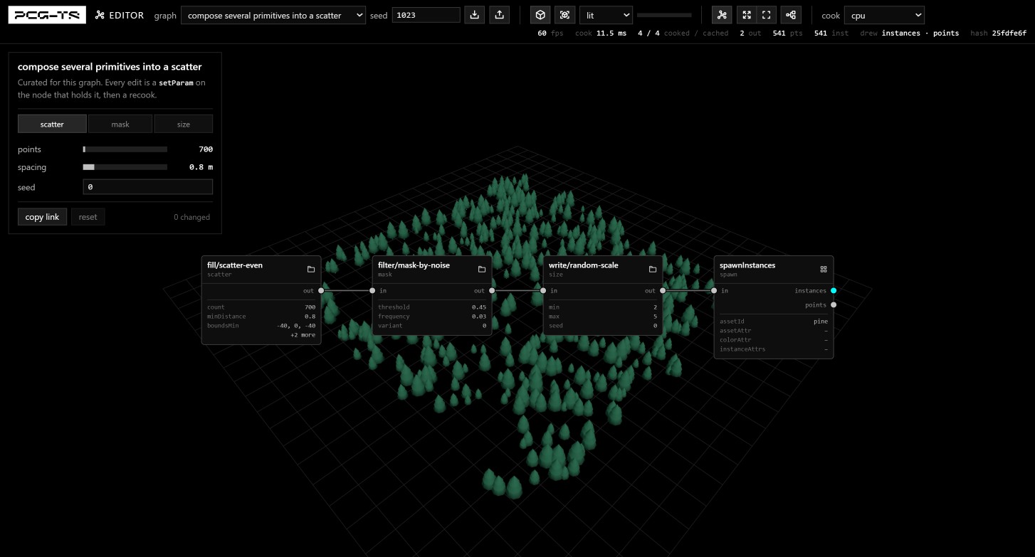
Tab summons the node menu wherever the pointer is. The shade control switches the render between a lit studio and surface normals — a redraw, not a recook — because the two answer different questions: lit says what a thing would look like, normals say what shape it IS, and a single key light flattens overlapping solids into one silhouette.The editor is the strongest existence proof the library has: it is built entirely on the same public API this manual documents. The palette — summoned at the pointer rather than parked in a column — groups by category from listNodeTypes(); the inspector renders each parameter from its schema, including whether it accepts a field; the description text under the node name is the registry's own prose. Import and export are deserializeGraph and serializeGraph verbatim. The knobs panel floating over the canvas is the one thing the registry does not supply: it is a per-graph panel spec under graphs/panels/, naming which params are worth a slider, and every edit it makes is a setParam on the node that holds it. Chapter 5 drives the whole tool.
The graph picker is the corpus. shared/presets.ts globs graphs/*.json for its menu, so a graph added to the corpus is a preset added here, and ?graph=<name> in the URL opens the page on one of them.
A field expression, as text
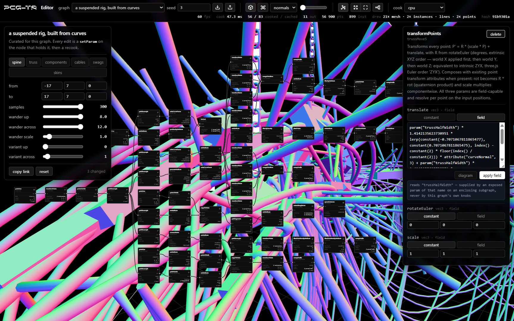
shade control is on normals, which is a redraw rather than a recook and answers what shape a thing IS where a lit key light would flatten the overlapping tubes into one silhouette. The knobs column is a per-graph panel spec, not the registry. And the inspector is showing a field expression as text — printFieldSpec on the way in, parseFieldText on the way out — where the same parameter once showed forty lines of nested JSON. The tree is still the format and is still what the file holds; the text is a view over it, so a knob turned anywhere else re-prints rather than fighting an authored string.One graph, three cook paths
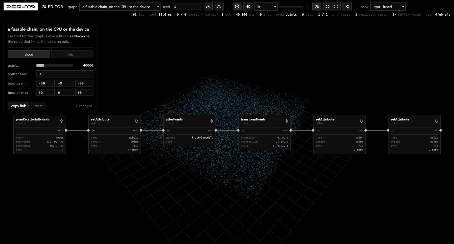
1 run / 2 fused and 1× suffix-fused mean four of the six nodes cooked node by node and only the last two became a device-resident run.The cook selector changes how the graph cooks and nothing about the graph. cpu passes no resolver at all, so its bytes and its memo keys are what they would be with no device in the machine; gpu · per-node is the evaluator behind a wrapper whose planRun returns null, so field params resolve on the device but nothing fuses; gpu · fused is the evaluator itself. Switching the selector and watching two numbers on the status line — the wall time and the hash — is the whole comparison, live rather than tabulated.
Measured on one adapter at the shipped 40,000 points, cooking examples-gpu-fields at seed 1: 485 ms on the CPU, 41 ms per-node, 35 ms fused. Run-to-run spread on the device paths is a few milliseconds either way — the capture above is a separate run and read 27.6 ms — so treat the ratio as the finding and not the third digit. Read them as steady-state numbers, too. The first cook on a device path is not one — it compiles pipelines, and the per-node path's first cook measured 293 ms against the 41 ms every cook after it. Pipelines are cached on the evaluator instance and persist across cooks, which is why the fused path never pays that entry fee separately: by the time you reach it, per-node has already compiled the member kernels it shares.
The hash holds across the two device paths and not across the CPU, and the page says so in the selector's own tooltip rather than leaving you to discover it. At seed 1 both device paths return 4fe04a4a and the CPU returns ca4b526f. That is the determinism contract working as designed, not a defect — chapter 6 sets out the shape of the difference, and docs/authoring.md records a measured maximum |cpu-gpu| of 1.19e-7. The invariant is same seed, same path. Agreement between per-node and fused is the one worth watching, because it is the one a change to the run planner could break.
The counters are the interesting half. 6 disp counts member kernels, not dispatchWorkgroups calls. 1 run / 2 fused is the plan the executor actually got: this chain does not fuse whole, because jitterPoints and transformPoints rewrite P ahead of two identity-keyed members, and a run may rewrite P or key on identity but not in that order — so the planner declines the run and the executor retries the suffix, recovering [color, psize]. 1× suffix-fused is reported apart from the fallback list for exactly that reason: it is a partial success, not a loss, and reading it under the same heading as compile-error would misfile it.
The graph ships at 40,000 points and the panel's ceiling is 200,000, which is about three seconds of blocked tab on the CPU path — as much as a page with no cook budget should be able to ask for. The demo this replaced ran at a million and took ten to twelve seconds per CPU cook. Blocked because this page cooks synchronously on the main thread, which is a property of the demo and not of the CPU path: pcg-ts/worker moves the same cook to a worker thread, and its results come back across the transfer list rather than as a copy. Read "CPU path" throughout this chapter as "not the GPU device" — never as "on your frame".
listNodeTypes · getNodeType · describeSubgraphPins · isField serializeGraph · deserializeGraph · fieldFromJson · fieldToJson mutation API: add · connect · disconnect · removeNode gpu: GpuFieldEvaluator · CookOptions.gpu · CookStats.gpu run it → the fusable chain →
Infinite world — hierarchical streaming
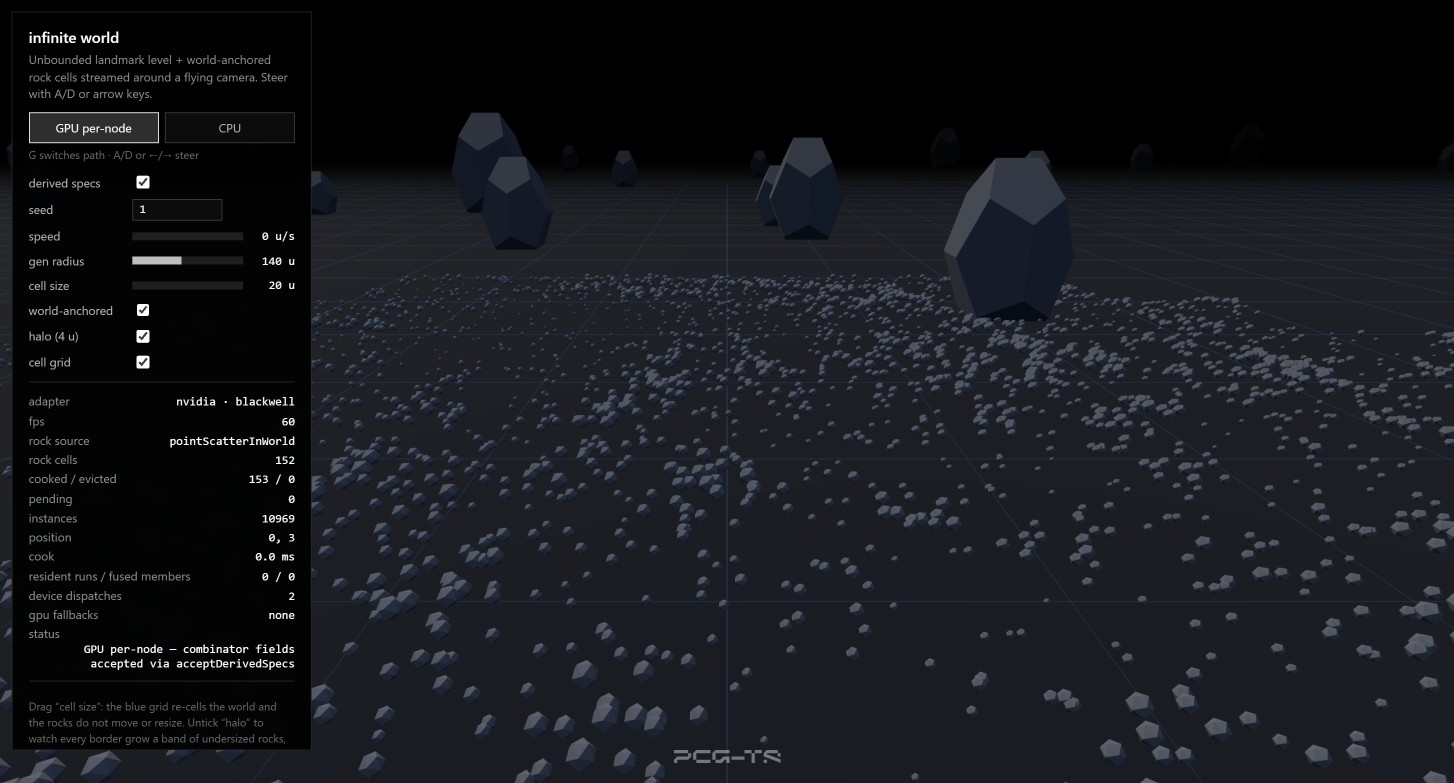
Two levels: an unbounded level holding the landmark boulders (one global cell, no radius), and a bounded level of small rocks that streams around the camera. The counters tell the streaming story directly — cells cooked, cells evicted, and a pending queue that stays at zero because update is called with a millisecond budget every frame. The screenshot catches it at rest, with the camera parked and nothing yet outside the radius: 155 cooked against 0 evicted. Fly, and the eviction counter starts moving while the live count holds steady.
Fly out to the edge of the generation radius and back, or drag the radius slider while moving, and the same rocks return in the same places. That is the order- and path-independence guarantee being exercised rather than asserted: the cell content never depended on the route.
The rock level is built on pointScatterInWorld, and each rock is sized by how crowded its surroundings are — a measurement that does not stop at a cell border, so the level asks for its cell grown by a halo, measures over that, and clips back with filterByBounds. Tick cell grid to draw the partition itself — the blue lines in the screenshot — and two more checkboxes turn the argument of 2.5 into something you can watch fail. Untick halo and every border grows a visible band of undersized rocks: the neighbourhood ran out of world. Untick world-anchored and the source becomes pointScatterInBounds — still perfectly deterministic, no longer anchored — after which dragging the cell size slider re-rolls the whole world instead of merely re-partitioning it. Anchored, that same drag moves and resizes nothing at all, which is the strongest single demonstration in the examples that the content is not a function of the runtime's partitioning.
Since v0.9 the panel also carries a GPU per-node / CPU toggle and a derived specs checkbox, and that checkbox is the tidiest demonstration of what v0.9 changed. Every field in this example is written with the combinator API — remap(randomField("mega"), 0, 1, 5, 13) and friends — which until v0.9 could not reach the device at all. Untick the box and gpu fallbacks reads derived-spec ×5 with zero dispatches; tick it and the fallbacks vanish and the dispatches appear. The instance count does not move either way, which is the point: the flag changes where the work happens, never what comes out.
What it does not show is fusion. resident runs / fused members reads 0 / 0 on both paths, and the demo has a why nothing fuses here section saying so: filterByDensity changes the point count and can never be a run member, which leaves both graphs as singleton chains, and a chain of one is only a run when it ends in a resident terminal. Reaching the device per node and fusing into one run are different wins, and this example is honest about which one it got.
World · LevelDef.bind · unbounded level · budgeted update pointScatterInWorld · ctx.worldSeed · halo query · filterByBounds (halfOpen) pointNeighborhood · setAttribute · filterByDensity · spawnInstances gpu: GpuFieldEvaluator · acceptDerivedSpecs · CookStats.gpu three: WorldThreeBinding run it →
Galaxy — determinism at scale
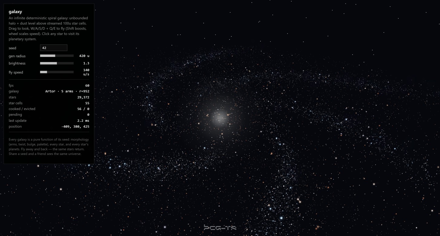
An unbounded halo and dust level above 100-unit star cells that stream around a free-flying camera. Everything is derived from the seed: the morphology (arm count, twist, bulge, palette), every star position and colour, and — one level further down — every planet of every star you click. The demo is really an argument about scope. A seed is a complete, shareable address for a universe, because nothing in it was ever a function of anything but the seed and the coordinate.
It also shows off the field grammar under load, composing atan2, ramp, length, trigonometry and simplex noise into the spiral density that decides where stars exist at all.
World · unbounded + bounded levels · per-cell seeding fields: atan2 · ramp · length · cos · clamp · gt · component · simplexNoise Pcg32 · hashCombine · transformPoints run it →
GPU world — matrices that never reach the CPU
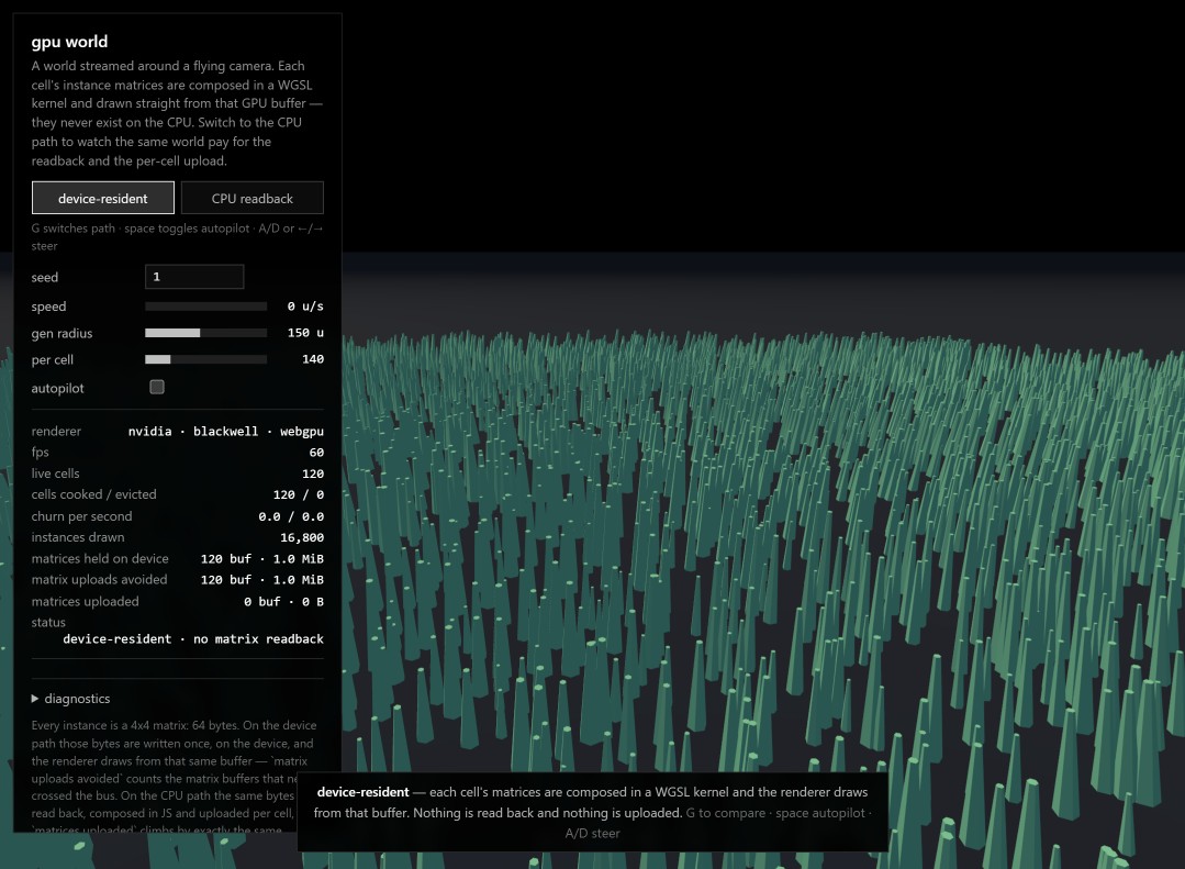
matrices uploaded row stays at 0 B for as long as the device path is selected.Where the editor's fused cook path keeps attribute columns device-side between fused kernels, this one keeps the result device-side as well. spawnInstances acts as the terminal of a resident run: the transform, scale and rotation columns stay in storage buffers, a WGSL kernel composes them into column-major 4×4 matrices, and the batch hands back an opaque buffer handle instead of a Float32Array. A renderer sharing the same GPUDevice adopts that buffer as a storage instance attribute, so the matrices go from compute kernel to draw call without ever existing in JS.
The toggle is the point of the demo. Both paths cook the same graph with the same fields on the same device — only the ending differs. Switch to CPU readback and matrices held on device falls to zero while matrices uploaded starts climbing; switch back and the upload counter freezes where it stopped. Both meters are cumulative, so they record what each path has cost since the page loaded rather than what it is holding right now. In the screenshot the camera is parked with autopilot off, nothing has evicted yet, and the cumulative buf count still agrees with live cells at 120; start moving and the two part company, which is the honest picture of a streaming world.
That divergence is also the leak check. Retained device bytes track live cells exactly — 120 cells of 140 instances is 120 × 140 × 64 = 1.0 MiB — while the cumulative counter climbs past it and keeps going. Handles are refcounted by identity, so a parent output aliased into several child cells is freed once, by the last cell to let go of it, in whichever order they evict.
One GPUDevice must back both the field evaluator and the renderer: a GPUBuffer belongs to the device that made it, two devices cannot share one, and a WebGL context cannot read a WebGPU buffer at all. Without that the demo says so in the status line and runs the CPU path instead of rendering something wrong. This level spawns one asset by choice, not by limit: assetAttr has been device-resident since v0.8.0 — no resident node can produce a string attribute, so the asset key is a host column by construction, the host plans the grouping with the same function the CPU spawner calls, and the device composes one buffer and one dispatch per asset in the identical batch order. The one spawner feature that is not device-resident is per-instance attribute channels: a spawn naming anything in spawnInstances' instanceAttrs rejects the whole resident run as run-plan-failed and the CPU spawner serves the entire terminal — transforms, colour and channels together — rather than a device run silently handing a host an ABI with holes in it.
The sentence above is about producing channels on the GPU device, and it is regularly misread as two other things it does not say. Rendering a custom channel under a WebGPURenderer is supported: the CPU batch carries every channel, and toInstancedMeshes binds each one as an InstancedBufferAttribute of its own name, with the column's dtype and derived item size intact. That function imports only three and branches on nothing renderer-shaped, so a WebGPU material reads the attribute exactly as a WebGL one does — it is the supported route for per-instance data in your shaders. The library ships the data and not the shader: nothing in it imports three/tsl or writes a material, and normalized/gpuType are left at three's defaults, so declaring the attribute (a TSL attribute() node, a ShaderMaterial, an onBeforeCompile patch) is yours to do. Only the device-resident adapter is narrower — it binds just the instance matrix and the reserved colour, and refuses a hand-built device batch carrying anything else rather than drawing without it. The cost to budget for is ownership, not throughput: an InstancedBufferAttribute lives on the geometry, so every batch carrying a named channel gets its own geometry clone — flagged by ownsGeometry(mesh) and yours to dispose with the mesh. Colour alone does not clone, since instanceColor hangs on the mesh instead.
Do not set gpuType on an integer channel. The advice going around — and two earlier versions of this claim in docs/authoring.md — says to, on the grounds that three defaults an attribute to FloatType. Measured instead, on a real draw call with a pixel readback (tests/instanceChannelRender.test.ts, in a browser — the u32 case under both renderers, the f32-column one under WebGL): a Uint32Array channel arrives exact with the flag untouched. WebGLAttributes maps it to gl.UNSIGNED_INT, and WebGLBindingStates chooses the integer pointer call as type === gl.INT || type === gl.UNSIGNED_INT || gpuType === IntType — the flag is the third disjunct, short-circuited before it is ever read — and the same ids come back byte for byte identical with it set and unset. It is load-bearing for an integer array narrower than 32 bits — Uint8Array, which is how a bool channel is stored, among them: gl.UNSIGNED_BYTE fails both type tests, so without the flag the pointer call succeeds and the draw fails, and such a channel wants declaring in uint rather than in int. And it is actively harmful on a Float32Array, where it makes three call vertexAttribIPointer with gl.FLOAT — not an accepted type there — and the driver answers INVALID_ENUM at the pointer call, which then does nothing. (Those last two are read out of three’s source and the WebGL2 rules; nothing in this repo binds them, so unlike the measured claims above they are not proven here — and note that three’s own JSDoc denies the second, calling gpuType “not configurable for float arrays” where the code has no such guard.) Nor does a mismatched shader declaration round quietly: a u32 channel declared in float gets the draw rejected loudly — a GL error, or no fragment at all, rather than a quietly wrong number, which is the pair the test pins rather than a code. The 2^24 collision is real, but it belongs to an f32 column and not to a missing flag — the same four ids carried through one read back [0, 0, 80, 160], two of them collapsed into one. That is what preserving the dtype across the spawner is for, and lanterns draws both columns of the same ids side by side.
And a CPU cook is not necessarily a main-thread cook. pcg-ts/worker cooks off-thread, and the encoded batch carries every named channel — colour among them, since colors is an accessor over the reserved entry rather than a second buffer. Every column rides the structured-clone transfer list, so the batch arrives on the main thread as buffer ownership rather than as a copy; the worker pays one slice per column on its own thread, because a cook's arrays alias live memo caches and must not be detached. A spawn that loses the device path therefore need not cost you a frame.
three: createWebGpuInstanceAdapter · WorldThreeBinding · DeviceInstanceAdapter gpu: GpuFieldEvaluator · deviceInstances · deviceTransformsBuffer run it →
The rig — the curve vocabulary, end to end
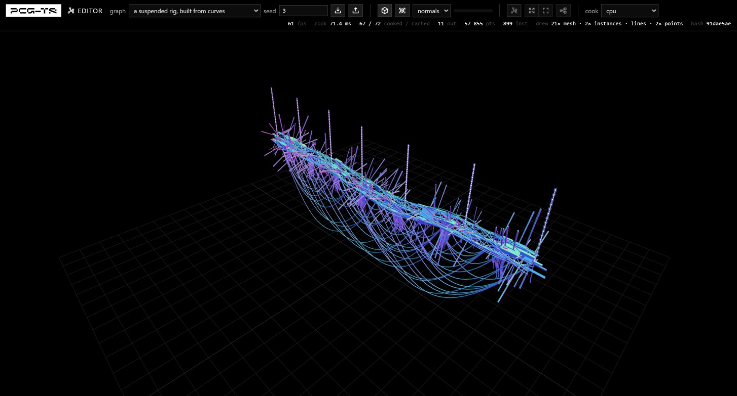
shade control is for: surface direction reads volume and overlap where a key light flattens them.This graph exists because of something the library could not do when it was written. meshPrimitive built planes and boxes, toLineGeometry emits a line one pixel wide, and there was no sweep or extrude — so a path could be generated and never drawn. pathSegments closed that without inventing a swept-surface representation: one instance point per polyline segment, at the midpoint, with rot turning the chosen axis onto the segment and scale carrying its length. A unit cylinder lands exactly on each segment, so every chord, brace and cable in the picture costs one draw call per group.
The rods point outward rather than all one way because of the second piece. orientAlongVector fixes roll with an up hint, and a constant up cannot follow a curve that turns over — as the tangent passes through it the roll flips a half turn and everything placed along the curve snaps round. writeCurveFrame carries a normal along the curve instead, transported point to point by double reflection, and up is field-capable so cos(a) · curveNormal + sin(a) · curveBinormal can be fed straight back in. The radial fan slider is that angle's range: at 0 every component lines up on one side, at a full turn they cover the circle.
Components mount to a CHORD rather than to the truss axis — a fixture on the centreline of a box truss is inside the box. The fan angle is snapped to the nearest corner and the point steps out there, so a fixture leaves from the tube it would really be clamped to while still pointing along its own fan angle. That angle is written to an attribute BEFORE the point moves and read back afterwards, which is not fussiness: randomField keys on point IDENTITY, so drawing it again after the move yields a different number and the chord a fixture sits on would disagree with the way it points. Which shape each point spawns comes from spawnInstances' assetAttr, written by a string setAttribute whose values list is weighted by repetition — which is why the mix grid takes integers. The cable bundles are pathPointAt: each anchor slides a fraction of the way toward the centre of its bin, expressed as lerp(curveU, centre, amount), so nothing is removed and the cable count is exactly what the slider says. The swags are connectPoints chords sagged by a parabola over the carried edgeLength, then thinned by length and by a per-chord random living on the primitive domain — thinning by length alone leaves a lattice, because every surviving pair still gets hung.
The truss is the frame paying for itself a second time. Its four chords are the SAME curve pushed sideways by h · (cos a · curveNormal + sin a · curveBinormal), the unit vector at angle a in the plane perpendicular to the tangent — and since transformPoints preserves topology, a displaced path is still a path and goes straight to pathSegments. Without a normal carried along the curve there is no stable "corner one" to run a chord down and the section would spin as the spine turned. A chord holds its angle; a brace alternates between two adjacent corners as it advances, which is what triangulates each bay. That alternation is station parity, and because parity is 0 or 1 the two angles are reached by lerping their cosines and sines rather than by evaluating trigonometry per point. The square cross-frames are not new geometry at all but a REGROUPING of points that already exist: mergePoints concatenated the four chords in connection order, so a point’s index is chord × stations + station — grouping by the index modulo the station count collects one point from each chord, in ascending chord order, which walks the square rather than crossing it.
The chains are the same three ideas turned once more. A chain link is an oblong ring — a tube swept around a stadium outline, which is what a real link is and what makes a chain read as a chain rather than a string of hoops — whose plane contains the chain, and consecutive links sit a quarter turn apart — both fall out of AIMING the torus rather than rolling it, since orientAlongVector puts its axis onto a horizontal direction and alternating that direction between two horizontal axes gives the quarter turn. Each link is scaled by its own segment's length, read back out of the scale that pathSegments just wrote, so chains spanning different gaps stay properly linked instead of gapping on the long ones and piling up on the short.
nodes: pathSegments · writeCurveFrame · pathPointAt · orientAlongVector · connectPoints primitives: place/radial-on-curve · transform/gather-on-path · write/curve-frame forEach: one body per cable, seeded on its carrier open it →
Chapter 5
Using the graph editor as an authoring tool
The editor is a tool, not a demo: it opens any graph in graphs/ and edits it live, and what it exports is the same JSON your application loads. Open it hosted — it takes ?graph=<name> — or run it locally with npm run examples. It carried a 01- prefix once, which is exactly what made it read as the first demo.
Everything chapter 4 says about it being built on the public API this manual documents is also the reason it is worth authoring in: there is no second implementation of anything here, so a graph that behaves in the editor behaves in your application.
What is on screen
Two layers, one over the other. The render is the cook you are looking at; the node canvas is a full-bleed overlay over it, not a pane beside it. The space bar cycles the three views — scene, scene + graph, graph only — and shift+space walks back. There is no fourth state with neither layer up, so clicking the toggle of the only layer showing swaps to the other rather than clearing the page. In the combined view the toolbar's slider pushes the render back until the nodes read over it, and the mouse is split between the two layers by what it is over rather than by a modifier — see below.
Two cards float over the canvas. One is the loaded graph's knobs — its title, what it is for, and the params worth turning — and it is always up, because every graph has some. The other is the node inspector, and it exists only while a node is selected: a panel that is empty most of the time is a panel asking for the width back. Cook errors get their own strip under the toolbar rather than a dialog, so the graph they are about is still in front of you.
The toolbar
Grouped by what each control touches, which is the distinction the bar is built around: frame points the scene camera and fit zooms the node canvas, and sitting side by side they read as a pair of the same thing when they are the same verb on opposite subjects. Every icon button keeps its word in its tooltip and its accessible name.
| Group | What is in it |
|---|---|
| The graph | graph is the corpus picker: shared/presets.ts globs graphs/*.json, so a graph added to the corpus is a preset added here, and ?graph=<name> in the URL opens the page on one. seed sets the graph seed. Export produces serializeGraph output; import takes pasted JSON through deserializeGraph. |
| The render | Its own on/off switch, then frame (point the camera at what the graph made), the shade selector — lit or normals — and the legibility slider. shade is a redraw, not a recook: lit says what a thing would look like, normals say what shape it is, and vertex colours only show under lit. |
| The node canvas | Its own on/off switch, then fit (zoom out until every node is on screen, however small), 100% (back to 1:1), and layout, which re-runs the deterministic topological layout. All three move boxes; none of them moves the camera. |
| The cook | cook selects the path — cpu, gpu · per-node, gpu · fused. It changes how the graph cooks and nothing about the graph, and the device entries are disabled until an adapter is up. |
The cook paths differ in exactly one way each. cpu passes no resolver at all, so its bytes and its memo keys are what they would be with no device in the machine; gpu · per-node resolves field params on the device but fuses nothing; gpu · fused is the real evaluator. The hash holds across the two device paths and not across the CPU — chapter 4 walks a live comparison and chapter 6 sets out the shape of the difference.
The status line
Under the toolbar, in one line: frames per second, cook milliseconds, nodes cooked versus cached, how many outputs the graph declares, points, instances, what was actually drawn, and an output hash. On a device path it grows the counters that path earns — dispatches, resident runs and fused nodes, readbacks saved, any suffix-fused count, and the fallbacks by reason. That is the same stats.gpu record chapter 6 describes, rendered rather than logged.
The hash is the fastest determinism check you have: same graph, same seed, same path, same hash. It is also what makes an import trustworthy — the toast after one quotes the output hash and says whether it matches the cook before it, so pasting a graph you believe is the same graph is a checkable claim rather than a hope.
Authoring a graph
- Summon a node with
Tab. The node menu opens wherever the pointer is rather than sitting parked in a column, grouped by the registry's own categories — source, sampler, surface, point op, filter, attribute, value, spawn, io, composite — so you find a node by what it does rather than by remembering its name. The search field takes focus as it opens, the arrows move the highlight andEnterplaces it:Tab, a few letters,Enter, without the hand leaving the keyboard. - Wire pins left to right. Inputs are on the left of a node, outputs on the right. The editor refuses invalid connections because it asks the live graph, and the live graph validates eagerly.
- Edit parameters in the inspector. Each parameter renders from its schema: enums become dropdowns with exactly the legal values, numeric parameters carry their documented range, and a field-capable parameter shows a
constant / fieldtoggle. In field mode the expression is written as text —printFieldSpecon the way in,parseFieldTexton the way out — and adiagrambutton draws that same expression, read-only, as boxes and wires whenever the text parses. No JSON appears in that widget at all. The tree is still the format and still what the file holds; the text is a view over it, which is what lets a knob turned somewhere else re-print the parameter rather than fight an authored string. - Declare what comes out. An unconnected output pin is a declared graph output — that is how you say "this is what I want out".
- Watch the status line. After an edit,
cookedshould be exactly the node you touched plus its dependents. More than that means something upstream changed that you did not mean to change. - Export. The button produces
serializeGraphoutput. Paste it intodeserializeGraphin your application and it cooks identically.
Deleting a node — the button in the inspector, or Delete with it selected — cascades: every connection touching it and every output declared on it go with it, in a single version bump. Watch the cooked-versus-cached counters when you do it. Untouched branches keep serving from cache, because the editor edits the live graph through the mutation API rather than rebuilding it from JSON. A rebuild is fully validated but starts cold; mutation is what keeps a large graph pleasant to edit.
Tuning a graph, and sharing the result
The knobs card is as much the pane you read to learn what a graph does as the one you turn. A graph that ships a panel spec under graphs/panels/ gets a curated panel, its sections as tabs, and one row there may stand for several params — four chord tubes are one "chord" setting. A graph that ships none gets a panel derived from the exposed params of its subgraph nodes, grouped by the node that exposes each. Either way a row writes setParam on the node holding the value, which is the same call the inspector makes, so the two views of one knob cannot drift. A graph exposing nothing says so and sends you to the canvas.
copy link writes a URL carrying the graph name and everything you moved — ?graph=<name>&p=<patch> — so a tuned state is shareable and reopens exactly, and the patch lands as one edit, so a twelve-knob link is still one recook. reset puts every knob and the seed back to what the graph loaded with. The N changed button beside them reveals the link and the patch itself, read from the live graph rather than from the panel, so a param you edited in the inspector — or one the spec chose not to surface — is in it too. The seed counts as part of the patch.
Keyboard
| Key | What it does |
|---|---|
Space | Cycle the view: scene → scene + graph → graph only. Shift+space walks back. |
Tab | Summon the node menu at the pointer, and close it again. Only while the graph is up — with the scene alone on screen there is nothing to add a node to, and Tab goes back to being the browser's. |
F | Re-frame the scene on what the graph made. The camera is placed when a graph loads and then left alone, so this is the way back after flying off, or after a knob has grown the content past the pose it was framed at. |
Ctrl/Cmd+0 | Put the node canvas back to 100% — the chord that resets zoom everywhere else. The 100% button is the same action. |
Delete / Backspace | Delete the selected node. |
Every one of those yields to a focused text field and to an open modal, so a space typed into a param box is a space. Ctrl+0 is the one exception, and for a reason rather than by omission: it means nothing inside a text field, so there is nothing to yield to and it still works with the caret in a param box.
The canvas itself pans with the right button and zooms on the wheel; a graph opens at 100% whenever it fits there and fitted otherwise.
The mouse, when both layers are up
In scene + graph the two layers want the same three gestures, and which one answers is decided per event by what is under the pointer — no modifier, and nothing to hold.
| Under the pointer | Left drag | Right drag | Wheel |
|---|---|---|---|
| A node's box | Move the node | Pan the whole graph | Zoom the graph |
| An output pin | Pull a wire out of it | Pan the whole graph | Zoom the graph |
| A wire, or an input pin | Nothing — a wire is clicked to cut it, and an input pin is a drop target | Pan the whole graph | Zoom the graph |
| The space between them | The scene, exactly as it flies with the graph turned off: orbit, pan, dolly. | ||
Wires and input pins count as graph, not as scene, even though a left-drag on one does nothing: a cable is what you click to cut, and an input pin is where a wire is dropped, so both keep a hit target and neither hands the drag to the camera. In graph only there is nothing behind the canvas to reach, so the canvas takes the whole surface and an empty right-drag pans as it always did.
Clearing the selection is the one place the two layers still overlap: a plain left-click on the render, like a left-click on empty canvas, closes the inspector. The scene's right and middle drags do not — panning the camera is not a statement about which node you were reading.
Chapter 6
GPU cooking
The GPU path is opt-in, additive, and honest about being an approximation. Nothing changes unless you pass a resolver into cook.
Turning it on
import { cook } from "pcg-ts";
import { GpuFieldEvaluator } from "pcg-ts/gpu";

const adapter = await navigator.gpu.requestAdapter();
if (!adapter) throw new Error("no WebGPU adapter");
const device = await adapter.requestDevice();
const gpu = new GpuFieldEvaluator(device, { adapterInfo: adapter.info });

const result = await cook(graph, { gpu });
console.log(result.stats.gpu);
// { dispatches, pipelinesCompiled, pipelineCacheHits,
//   residentRuns, fusedNodes, readbacksSaved, fallbacks: {...} }
The core never imports the GPU module — the graph layer sees only a structural resolver interface, injected per cook. The same option exists on WorldOptions.gpu and UpdateOptions.gpu (update wins), threading a resolver into every cell cook.
What actually compiles
The GPU surface is exactly the serializable field-expression grammar, and all of it compiles: inputs, arithmetic, trigonometry, clamp/lerp/remap/select/ramp, vector operations, and every noise family including fBm and exact worley. The dividing line is not which functions but how the field was built. A field built by fieldFromJson carries a spec and is eligible; a field composed from the code combinators has no spec and stays on the CPU. getFieldSpec(field) tells you which you have — it returns the spec, or undefined.
Six nodes resolve their field parameters on device: setAttribute, transformPoints, jitterPoints, orientAlongVector, surfaceSample and volumeSample. Subgraph nodes forward the resolver to their inner cooks. Element count is never a limit — a kernel covering more elements than one dispatch call allows splits into chunks with byte-identical output.
When a field cannot run on device it falls back to the CPU silently but countably. stats.gpu.fallbacks records machine-readable reasons, and the vocabulary is closed: no-spec, compile-error, too-many-buffers per field, and run-plan-failed, run-too-large, run-partially-fused per fused run. If you expected device execution and did not get it, that record names why. The last of those is a partial success rather than a lost run: a member was rejected, the planner retried the suffix after it, and what remained fused — so read it together with residentRuns and fusedNodes, which say how much of the chain the retry recovered.
Device-resident runs
Beyond per-node evaluation, the executor finds maximal linear chains of fusable nodes and cooks each as a single device round trip. Four node kinds fuse — setAttribute in numeric point-domain mode, transformPoints, jitterPoints and orientAlongVector — all count-preserving, one geometry in and one out. A run ends at a non-fusable node, at any fan-out, and at a node carrying a declared graph output. A chain of one is not a run.
Fusion never changes which bytes the rest of the graph observes: an interior node with external consumers simply becomes a run terminal with its own readback. Only the terminal caches, under a composite key covering every member in order, so editing any member recooks exactly that run and leaves siblings and upstream cached.
The determinism contract, in plain language
The CPU is the bit-exact reference and existing goldens never move. The GPU is a documented approximation of it, and the shape of the difference is this:
- Integer work is bit-exact. Hash and random streams, noise lattice hashing,
index, integer attribute reads, boolean-to-float reads, and pure hash-compare-select trees all produce byte-identical results on both paths. - Float work matches within measured budgets. The CPU computes in f64 and stores f32; WGSL computes in f32 throughout. Addition, subtraction, multiplication,
clamp,min/max,floor,fract,mod,sign,smoothstepand comparisons are bit-exact anyway. Division,lerp,remap,dotanddistancestay within one range-ULP;rampandlogwithin two; vector length within four;powandexpwithin eight, which is the widest of the algebraic functions; sine and cosine within twelve; the inverse trigonometric functions are the loosest, as the WGSL specification permits. Noise families sit between six and twenty-four depending on base and mode. The full table lives in llms.txt and docs/authoring.md. - On one device, repeated runs are byte-identical. The variability is between the CPU and the GPU, and between different adapters — not between two runs on the same machine.
- Branchy operations can flip. Comparisons,
select,rampsegment boundaries and worley cell walks may take the other branch at knife-edge inputs whose operands differ within tolerance. A point right on a filter threshold may survive on one path and not the other. - Every budget was measured on one adapter. Another adapter exceeding one is a finding worth reporting, not expected noise.
Because GPU output is not byte-identical to CPU output, cache provenance folds the resolver's cacheSalt — a format version plus the adapter's identity — into the memo key of any node that would resolve a live spec'd field on device. Toggling the GPU on and off therefore never serves bytes produced by the other path. It also means the chain recooks on every flip, because a node holds one memo slot. That is by design, and it is why every benchmark in chapter 4's cook-path comparison is a cold-cache cook.
When it helps, and when it does not
The GPU path pays off when the same field expression is evaluated over a very large domain — hundreds of thousands of elements and up — and pays off most when several such nodes sit in a fusable line, because then the readbacks disappear too. The examples-gpu-fields chain at a million points — the size the page it replaced ran at — was roughly twenty times faster than the CPU reference on one desktop adapter, on both device paths, with the fused path keeping only the tail of the chain resident and cooking the rest per node.
It does not help, and can cost, when the domain is small enough that dispatch and readback dominate; when the fields were composed in code and carry no spec, so every one of them falls back; when the graph's cost is in topology rather than fields, since only field evaluation moves to the device; or when you are toggling the path back and forth, which recooks the chain each time. Bit-exactness with existing goldens is a reason to stay on the CPU, and staying on the CPU is always a supported choice — it is the reference.
What is on device today is field evaluation, plus fused runs of the four count-preserving node kinds above, plus one terminal kind: spawnInstances. Under deviceInstances: true a run can end at the spawner and compose its 4×4 matrices — and, with colorAttr set, its per-instance RGB — straight into GPU buffers a WebGPURenderer draws from, with no readback at all; multi-asset spawning has been device-side since v0.8. Chapter 4's gpu-world demo runs it, and docs/authoring.md carries the contract. Anything beyond that — topology, sampling, spawner-side allocation — is unshipped. Named per-instance channels (instanceAttrs) are unshipped on this list in one specific sense: the device compose kernel does not produce them, so a spawn naming one falls back to the CPU spawner. They are fully available as data and fully renderable — including under a WebGPURenderer, via toInstancedMeshes — and the cook can run off-thread through pcg-ts/worker. See the box in chapter 4 for the distinction, which is easy to lose.
Chapter 7
Debugging a graph
Cook stats are the first thing to read
Every cook returns stats: { cooked, cached, elapsedMs }, and the ratio answers most "why is this slow" questions immediately. A graph that recooks everything on every frame has a cache-invalidation problem, not a performance problem. Common causes, in rough order of frequency: a parameter is being set to a freshly constructed array or field every frame, so its structural hash changes; a dataInput node is being rebound with a new items array when the data has not changed; or a field is being rebuilt from JSON per frame instead of once.
The inverse reading is just as useful. After an edit, cooked should be exactly the edited node plus its dependents. If it is more, something upstream is changing that you did not intend to change.
Cache hits after an edit — a real trace
await cook(graph);                          // { cooked: 4, cached: 0 }  — 1008 survivors
graph.setParam(density, "value", fieldFromJson(newSpec));
await cook(graph);                          // { cooked: 3, cached: 1 }  —  967 survivors
One node cached: the scatter, which is upstream of the edit. Three cooked: the edited node and the two that depend on it. That is exactly the contract, and seeing it hold is how you confirm a graph is wired the way you think it is.
Determinism is a debugging tool, not only a feature
Because the same seed produces the same bytes, a hash of an output column is a stable fingerprint. The editor prints one in its status line for precisely this reason. Hash your output, change nothing, cook again, and compare: if the hash moved, something in your pipeline is reading state you did not declare — wall-clock time, an unhashed external array, Math.random somewhere in your own code. If the hash is stable but the picture is wrong, the bug is in the graph, and you can bisect it by declaring an output on an intermediate node and cooking only that one.
The same property makes bug reports reproducible in a way that is otherwise rare in procedural work: a seed and a serialized graph fully determine the output.
What the error messages already tell you
Error strings in this library are treated as part of the API surface: they name the offending node, pin or parameter, and they list the valid alternatives instead of leaving you to search for them. Reading the message is usually faster than reading the code. Chapter 11 shows the real strings and how a program should react to them; for a human the practical advice is shorter — the message names the thing, and the second half of the message is the fix.
The typed classes let you distinguish causes when you need to: GraphValidationError (bad structure or unknown pins), GraphCycleError, NodeExecutionError (carries .nodeId), CookCancelledError, GraphSerializationError, FieldJsonError, and WorldValidationError.
Five contracts whose violations are invisible
Most confusing behaviour in practice comes from one of five contracts, each of which fails quietly rather than loudly:
- Cook results are immutable. They alias live cache internals. Mutating one corrupts the cache with no error — clone first with
cloneGeometry. - Removing points destroys topology. Every filter that can drop a point rebuilds the point domain from the survivors and loses primitive topology with it, as do
mergePointsandpartitionByAttribute; only a node that clones preserves it. So a path that passes through one stops being a path — silently, where it happens, surfacing much later as a path consumer reporting that it found no polylines. A network fromconnectPointsfares worse, because nothing downstream necessarily complains at all: afilterByBoundsplaced after it reads like trimming the net to a rectangle and is actually demolition, and the cook succeeds with a plain point cloud where a road network was. Build the topology after the last filter, not before it; when the clip is a partition boundary rather than an authoring choice, own each edge by its lower-keyed endpoint on the primitive domain instead of filtering points at all. - Bound arrays are frozen by convention. An array bound into a parameter is captured by reference. Mutate it in place and stored cell outputs change with no staleness signal. Bind a fresh array.
- Columns are transient. An evaluated column may alias attribute storage and is only valid until the geometry is mutated or resized.
- Do not edit a graph mid-cook. Edits during an in-flight
cookorWorld.updateare detected and heal on the next pass — but that pass may return a torn mix of old and new state.
Chapter 8
Runtime capability discovery
The registry is the truth. Node types are not a list in the documentation that the code happens to match — the documentation is generated from the registry, so anything you can read in docs/nodes.md you can also ask for at runtime.
There are three registries, and an agent should know all three before emitting anything: listNodeTypes() for node types, listFieldFns() for the field-expression vocabulary, and listSubgraphs() for the named primitives — the ready-made recipes a graph can reference by name instead of rebuilding. Each has a generated twin on disk and a pcg subcommand that prints the same thing from a shell.
listNodeTypes()
Returns every registered node type. Each entry has exactly these keys: type, description, category, inputs, outputs, params. There are 61 types in the standard library, all categorized.
import { listNodeTypes } from "pcg-ts";

const types = listNodeTypes();
types.length;                                // 61
const jitter = types.find(t => t.type === "jitterPoints");
The entry, verbatim
{
  "type": "jitterPoints",
  "description": "Offsets each point by a deterministic random vector: each axis
    moves by a uniform random in [-amount, +amount], hashed from (seed, point
    index, axis) — order-independent and reproducible. amount is field-capable
    (evaluated on the input positions; tuple 1 broadcasts to all axes).",
  "category": "point op",
  "inputs":  [ { "name": "in",  "kind": "geometry", "multi": false } ],
  "outputs": [ { "name": "out", "kind": "geometry", "multi": false } ],
  "params": {
    "amount": {
      "type": "vec3",
      "default": [0.1, 0.1, 0.1],
      "description": "Maximum offset per axis, in world units. Field-capable (tuple 1 broadcasts).",
      "acceptsField": true
    },
    "seed": {
      "type": "u32",
      "default": 0,
      "description": "Extra seed folded into the node seed; change it to re-roll the jitter."
    }
  }
}
That is everything needed to emit a valid node: the type name, which pins exist and what kind they are, which parameters are legal, their defaults, and — critically — acceptsField, which tells you whether a field spec object is allowed in that slot. Parameter schemas additionally carry min / max for numeric ranges and enum for enumerated values, which is how the editor knows to render a dropdown containing exactly the legal strings.
Categories
Every standard type declares a category, so a palette or a generated document groups without heuristics. The grouping as of this writing — listNodeTypes() is the authority, and docs/nodes.md is generated from it:
| Category | Types |
|---|---|
source | pointGrid, pointLine, pointScatterInBounds, pointScatterInWorld, meshPrimitive, meshFromField |
sampler | surfaceSample, splineSample, volumeSample, pathResample |
point op | pointsToPath, connectPoints, transformPoints, jitterPoints, copyToPoints, mergePoints, orientAlongVector, setBounds, voronoiCells |
filter | filterByDensity, filterByBounds, filterByAttribute, filterByExpression, filterPrimitivesByBounds, selfPrune, projectToPlane |
attribute | writeTangents, pointNeighborhood, sampleNearestPoint, setAttribute, promoteAttribute, transferAttribute, attributeReduce, attributeRemap, removeAttribute, partitionByAttribute |
value | valueConstant |
spawn | spawnInstances |
io | dataInput |
composite | subgraph |
Building a graph in code from a type name
Two companions make the registry usable as a factory, not only as a catalog. hasNodeType(name) is a boolean existence check. getNodeType(name) returns { def, info } — info is the same metadata entry listNodeTypes() yields, and def is the node definition you can hand straight to graph.add. It throws on an unknown name (listing every registered type) rather than returning undefined, so check first if the name came from somewhere untrusted.
import { Graph, cook, getNodeType, hasNodeType, firstGeometry } from "pcg-ts";

if (!hasNodeType("pointGrid")) throw new Error("not registered");
const { def, info } = getNodeType("pointGrid");
info.type;                                // "pointGrid"

const g = new Graph(5);
const n = g.add(def, { countX: 3, countZ: 3 });   // n.id === "pointGrid_0"
g.output(n, "out", "p");
firstGeometry((await cook(g)).outputs.p).pointCount;   // 9
Note the generated id: a code-built node is named <type>_<n>, whereas a node loaded from JSON keeps the id you gave it. Both appear verbatim in error messages and in describe(), so meaningful ids in your documents pay for themselves the first time something fails.
listFieldFns()
Returns the complete field-expression vocabulary as a sorted array of 64 names. This is the closed set — an fn not in this list is not a field function, and emitting one produces the error in chapter 11.
["abs", "acos", "add", "asin", "atan", "atan2", "attribute", "attributeIs",
 "byAttribute", "clamp", "component", "constant", "cos", "cross", "distance",
 "div", "dot", "eq", "exp", "exp2", "fbm", "floor", "fract", "fraction", "ge",
 "gt", "index", "le", "length", "lerp", "log", "log2", "lookup", "lt", "max", "min",
 "mod", "mul", "ne", "nodeSeed", "normalize", "param", "perlinNoise",
 "position", "pow", "ramp", "randomField", "randomFrom", "rem", "remap", "select", "sign",
 "simplexNoise", "sin", "smoothstep", "sqrt", "step", "sub", "tan",
 "trunc", "valueNoise", "vec", "worleyFeature", "worleyNoise"]
listSubgraphs()
The third registry, and the one an agent gains most from: the named primitives. A primitive is a registered subgraph — a tested recipe with exposed params — that a graph references by name rather than rebuilding out of node types. 37 named primitives ship with the library, and listSubgraphs() returns them as { name, subgraph, hash, meta }: the canonical payload, its content hash, and a meta block whose title and description say what the recipe is for and how its knobs behave.
One thing about it is unlike the other two registries and will otherwise cost you an afternoon. Primitives register on import of their own subpath, so listSubgraphs() returns an empty array until something imports it:
import "pcg-ts/primitives";              // registers the whole catalog, as a side effect
import { listSubgraphs } from "pcg-ts";

const all = listSubgraphs();
all.length;                            // 37
all.find(s => s.name === "fill/scatter-even").hash;   // "3a0d277f9d3b1840"
That is a cost boundary rather than an oversight: import "pcg-ts" keeps costing nothing, and the catalog sits behind a subpath nobody pays for unless they want it. The pcg CLI imports it for you, which is why pcg run fill/scatter-even works on a clean install. Names are <family>/<kebab-case> over a closed set of seven families — shape, fill, transform, compose, filter, place, write — and the family is a promise about the pin shape. Node types are camelCase with no separator, so a name containing / can never be mistaken for a type. Chapter 9 covers how a graph references one.
The same catalogs, from a shell
Two of those registries are also commands. The pcg CLI is the library's other front door — npx pcg … when the package is installed, node bin/pcg.mjs … from a clone — and its discovery commands read the same registries this chapter has been calling:
# the whole registry, grouped by category
pcg nodes                      # -> "61 node types, by category"

# one type: its pins and its full param table, with ranges, enums and
# which params accept a field
pcg nodes pointGrid

# the field vocabulary, and one fn's allowed keys
pcg fields                     # -> "64 field fns"
pcg fields randomField         # -> usage: { fn: "randomField", key?: 0 | "salt" }

# every command takes --json and prints the machine-readable report instead
pcg nodes pointGrid --json
Two properties make this usable as a tool rather than as a convenience. Every command emits both renderings — a text one and, under --json, a structured one built from the same data — so the human reading a terminal and the agent parsing stdout are looking at one run and cannot disagree about it. And the exit codes are scriptable: 0 did what was asked, 1 a named thing does not exist or the run failed, 2 the command line itself was wrong. The distinction in the last two is the useful part — a graph that does not cook and a flag you spelled wrong are different problems and never share a code.
The primitives have no discovery subcommand of their own — they are read from docs/primitives.md, and pcg run <name> lists every registered name when it does not recognize one. Cooking a primitive standalone is pcg run too: pcg run shape/disc --param count=400 --param size=24,0,24 synthesizes a one-node wrapper around it and needs no graph file at all, which makes it the fastest way to find out what a primitive actually produces before committing a ref to a document.
The rule the graph-authoring skill states, and the reason these commands exist: never write a param name from memory. pcg nodes <type> costs a second and the deserializer will reject the guess anyway.
The generated catalogs, offline
If you would rather load a catalog than call into the library — for planning, for prompt context, for validating candidate graphs before a runtime exists — each registry has a generated file beside it. All of them ship inside the npm package, all are regenerated from the code (npm run docs), and none is ever hand-edited.
| Prose | Machine-readable | What it indexes |
|---|---|---|
| docs/nodes.md | docs/nodes.json | Every node type: pins, params, defaults, ranges. The JSON is a plain top-level array of the same 61 entries in the same shape listNodeTypes() returns. |
| docs/primitives.md | docs/primitives.json | Every named primitive: its pins, its exposed params with their derived schemas, its content hash, and a pcg run line to cook it standalone. |
| docs/graphs.md | docs/graphs.json | The example corpus: 95 graphs under graphs/, indexed by what each one teaches, with its tags, seed, node types and referenced primitives. |
The corpus is worth a sentence of its own, because it is the cheapest way to start. Every file in it teaches exactly one thing, carries a meta block saying which thing, and cooks from JSON alone — none uses dataInput, whose items never survive serialization — so any entry can be copied, cooked and modified with nothing but the CLI. Reading one graph near your goal and copying its shape beats composing from schemas.
Before emitting a graph: check whether a primitive already does it (docs/primitives.md opens with a one-line summary of each) — referencing one is a single node and it arrives tested. Then, for anything you are wiring by hand: confirm the type exists (hasNodeType, or pcg nodes <type>), confirm each parameter name is in params, confirm enum values against enum and numbers against min/max, confirm a field spec is only used where acceptsField is true, and confirm pin names against inputs/outputs. Every one of those checks the deserializer will also make — but making them first turns a thrown error into a corrected emission.
Chapter 9
Authoring graphs as JSON, end to end
The format
SerializedGraph, format version 1. Field names exactly as written:
- formatVersion
- Always
1. - seed
- Number. The graph seed; every node seed derives from it.
- meta
- Optional
{ title, description, tags }. The only place descriptive text belongs — there is no comment or annotation key. It is excluded from the content hash and does not bump the graph version, so retitling a graph cannot invalidate a cache. - params
- Optional array of graph-scoped params,
{ name, value, min?, max?, description? }each, in declaration order. One value declared once at the top level, read by name from any node's field expression as{ "fn": "param", "name": "tubeRadius" }with no inlinevaluebeside it — the shape for an authored quantity that occupies six nodes of one document. Binding happens at deserialize, by substitution into the expression, so the graph cooks byte-identically to one with the number written out in every reading slot. Written only when non-empty. See One value, many nodes. - nodes
- Array of
{ id, type, params }.idis yours to choose and is what every error message and every introspection read will call the node. Omitted parameters take their schema defaults. Asubgraphnode additionally carries either asubgraph: { graph, inputs, outputs, params }payload — the inner graph recursively in this same format, plus the exposed pin mappings and param declarations — or arefnaming a registered primitive. The two are mutually exclusive, and no other node type may carry either. - connections
- Array of
{ from: [nodeId, outputPin], to: [nodeId, inputPin] }. Order matters onmultiinputs: it is part of determinism. - outputs
- Array of
{ id, pin, name }.namebecomes the key inresult.outputs.
The format is closed, at every object position. An unrecognized key is an error, not something quietly ignored — inside the graph object, a node, a subgraph payload, a ref, a connection, a declared output, an exposed-pin or exposed-param declaration. This matters more to a generator than to a person, because the near-miss is the dangerous case: "refs" for "ref" under a lenient reader would have cooked as an ordinary subgraph node and reported success. The consequence is deliberate and permanent — a future field an old reader could misread arrives with a formatVersion bump, never by riding along unnoticed:
deserializeGraph: unknown key "notes"; valid keys: formatVersion, seed, meta,
params, nodes, connections, outputs. The format is closed — an unrecognized
key is a typo, not an extension, so a future field arrives with a formatVersion
bump. There is no annotation key: descriptive text belongs in the graph's
"meta" block ({ title, description, tags })
That is narrower than "a future format field", and the narrowing is the honest statement of what the rule protects. An added key is not the hazard it was written against: the list is closed, so an old reader meeting params refuses it by name rather than ignoring it, and nothing rides along. meta arrived that way, then the inline value on a param spec node, then params — all at format version 1. The bump is not free either: the subgraph content hash covers formatVersion, so moving it moves every pinned ref in the corpus. Spend it on a change to what an existing key means.
A complete working example
This document deserializes, cooks, and round-trips as written. It scatters two thousand points over a hundred-unit square, writes a normalized four-octave fBm into the density attribute, keeps points probabilistically against that density, and spawns the survivors.
{
  "formatVersion": 1,
  "seed": 7,
  "nodes": [
    { "id": "scatter", "type": "pointScatterInBounds",
      "params": { "count": 2000, "boundsMin": [0, 0, 0], "boundsMax": [100, 0, 100] } },

    { "id": "density", "type": "setAttribute",
      "params": {
        "name": "density", "domain": "point", "type": "f32", "tupleSize": 1,
        "value": { "fn": "fbm", "base": "perlinNoise",
                   "opts": { "frequency": 0.03, "octaves": 4, "normalized": true } }
      } },

    { "id": "keep", "type": "filterByDensity", "params": { "mode": "probabilistic" } },

    { "id": "spawn", "type": "spawnInstances", "params": { "assetId": "rock" } }
  ],
  "connections": [
    { "from": ["scatter", "out"], "to": ["density", "in"] },
    { "from": ["density", "out"], "to": ["keep",    "in"] },
    { "from": ["keep",    "out"], "to": ["spawn",   "in"] }
  ],
  "outputs": [
    { "id": "keep",  "pin": "out",       "name": "points" },
    { "id": "spawn", "pin": "instances", "name": "instances" }
  ]
}import { deserializeGraph, serializeGraph, cook, firstGeometry } from "pcg-ts";
const graph = deserializeGraph(doc); // validates everything, names any fault
const result = await cook(graph);
firstGeometry(result.outputs.points).pointCount; // 1038
result.stats; // { cooked: 4, cached: 0, elapsedMs: 13.8 }
const batch = result.outputs.instances
.find(i => i.kind === "instances").batches[0];
batch.assetId; // "rock"
batch.count; // 1038
batch.transforms.length; // 16608 (16 floats per instance, column-major)What round-tripping actually guarantees
This is the one place where an imprecise mental model causes real trouble, so be precise. serializeGraph(deserializeGraph(doc)) is not byte-identical to doc. Deserialization applies schema defaults, and serialization emits the full parameter set — so a node you wrote as { "count": 500 } comes back as { "count": 500, "boundsMin": [0,0,0], "boundsMax": [1,1,1], "seed": 0 }.
What is guaranteed is the pair of properties you actually need:
- Semantic fidelity. The round-tripped graph cooks byte-identically to the original.
- Idempotence after normalisation. Serialize once and you have the canonical form; serializing again produces exactly the same JSON.
JSON.stringify(s1) === JSON.stringify(s2)wheres2 = serializeGraph(deserializeGraph(s1))— verified.
So the correct diffing strategy for an agent is: normalise both sides through one serialize before comparing. Comparing your hand-written emission against a serialize output will report differences that are not differences.
One value, many nodes: graph-scoped params
One authored quantity is rarely written once. A cable radius reaches three nodes, a truss half-width twenty slots across ten, and the document then holds twenty independent numbers that a person has to keep equal by hand. The top-level params array is where that quantity lives instead: declared once, read by name from any node's field expression.
{
  "formatVersion": 1,
  "seed": 7,
  "params": [
    { "name": "tubeRadius", "value": 0.035, "min": 0.005, "max": 0.2,
      "description": "Radius of every tube in the rig, in metres." }
  ],
  "nodes": [
    { "id": "grid", "type": "pointGrid", "params": { "countX": 8, "countZ": 8 } },

    { "id": "thicken", "type": "transformPoints", "params": {
        "scale": { "fn": "mul", "args": [{ "fn": "param", "name": "tubeRadius" }, 2] } } },

    { "id": "lift", "type": "transformPoints", "params": {
        "translate": { "fn": "vec", "args": [0, { "fn": "param", "name": "tubeRadius" }, 0] } } }
  ],
  "connections": [
    { "from": ["grid", "out"],    "to": ["thicken", "in"] },
    { "from": ["thicken", "out"], "to": ["lift", "in"] }
  ],
  "outputs": [ { "id": "lift", "pin": "out", "name": "points" } ]
}
A reading slot writes the reference and nothing else — { "fn": "param", "name": "tubeRadius" }, with no value beside it. Binding happens at deserialize, by substitution into the expression, which is the same contract an exposed param has and the reason it is invisible to the cache in the right way: what comes back from deserializeGraph is an ordinary field with the number already inside it, so the declared graph cooks byte-identically to one with 0.035 written out in both slots. Cooking is untouched, and there is no per-cell or per-context channel through which two readers could see different values.
Turning one re-keys exactly the readers. graph.setGraphParam("tubeRadius", 0.05) rebuilds every authored spec that names it; a non-reader's params are not touched, so its memo key does not move and the next cook serves it from cache. The declared min/max binds that write, componentwise — the graph enforces its own range, because a hoisted value has no spec of its own to be refused by and a knob free to write past its stated maximum would make the range a decoration.
One name, one value. An inline { "fn": "param", "name": "tubeRadius", "value": 0.04 } in a graph that declares tubeRadius is refused at deserialize, naming both sites and both fixes. It is not a precedence rule: a graph-scoped param is the same document as the expression reading it, so an always-overridden inline value is dead text and a second address for one number. The rule that a binder beats an inline value still holds where it was written for — a subgraph binding a body, which is two documents, and where the body must also stand alone.
The rest, briefly. value is a literal — a finite number or a non-empty array of them, never a spec and never a reference to another param. It is an array rather than an object so that a repeated name is detectable, since JSON.parse collapses duplicate object keys before any reader sees them. A name may not contain a . or start with $, because the address is "$<name>" — one segment and a sigil, colliding with neither "<node>.<param>" nor the editor's bare "seed". A declared name nothing reads is legal and reported rather than refused (it is what a rename leaves behind; pcg validate --params prints it as read by nothing). And a subgraph payload's inner graph may not declare params at all: a body's names are bound by its wrapper's exposed params, which is the one binder it has, and a graph-scoped value reaches a body one hop at a time through the wrapper's own param slot.
describeGraphParams publishes the graph-scoped rows first, in declaration order, each carrying the address of every slot that reads it:
pcg validate rig.json --params

params:  12 addresses, 1 declared worth turning (*)
  1 graph-scoped param first, addressed "$<name>" — one value, every slot that reads the name
  the graph's own seed is a knob too, addressed as "seed" (currently 7)

  *  $tubeRadius          f32   0.035    0.005..0.2  read by 2 slots: thicken.scale, lift.translate
     grid.countX          i32   8        >= 1
     ...
Referencing a primitive instead of writing one
Everything above assumes you are wiring node types by hand. Often you should not be. A subgraph node can name a registered primitive instead of carrying a payload, and then the whole recipe is one node:
{ "id": "ground", "type": "subgraph",
  "params": { "count": 400, "size": [24, 0, 24] },
  "ref": { "name": "shape/disc" } }
For a generator this is the highest-leverage line in the chapter, and the reason is arithmetic rather than aesthetic: a reference is three keys where the equivalent embedded payload is an entire nested graph, so every primitive that fits collapses a passage of JSON you would otherwise have to emit correctly, and it arrives already tested with defaults tuned to produce something on the first cook. params on a ref node are the primitive's exposed params — not the inner nodes' params — and naming one that is not exposed is refused with the exposed set listed. docs/primitives.md and pcg run <name> are the two ways to find out what a given primitive exposes. Reach past a primitive to raw node types when it does not offer the pin or the param you need, not because a flat graph looks cleaner; it does not, it just loses the tests.
What is registered is a recipe, never a live graph, and every reference materializes a fresh copy through the same path an embedded payload takes. So the contract is the one you want: a reference and an embedded copy of the same recipe cook byte-identically — same output bytes, same cache decisions. Resolution happens once, at load, which also means a name must be registered before any graph referencing it is deserialized. Import pcg-ts/primitives first (chapter 8); the CLI does it for you.
Why the hash is optional
ref takes an optional second key, hash — the primitive's content hash, as returned by listSubgraphs() or registerSubgraph. Including it is a decision, not decoration, and the two modes are the whole design:
hash | What you are asking for | When the primitive changes |
|---|---|---|
| absent (the default) | "give me the library's current shape/disc" | Resolves and cooks. No friction — the graph gets the improvement. |
| present | "cook exactly what I authored against" | Hard error, naming both hashes. |
Optional is the load-bearing word, and it points both ways. Mandatory pinning would mean every improvement to a shipped primitive breaks every saved graph that references it — so a name-only reference is the default precisely so that it can upgrade freely. But there is no third mode, because neither mode warns. A library warning lands in a CI log or a console that the agent driving the graph never reads, which makes "resolve and warn" operationally indistinguishable from resolving silently — exactly the class of failure the determinism pillar exists to exclude. So: omit the hash while a graph is being developed against a library you control, add it when the graph is an artifact whose output you have recorded and intend to reproduce.
One boundary is worth knowing before you rely on a pin. The hash, and the byte-identity between the by-name and embedded forms, hold within one build. Across library versions neither can, by any design — an embedded payload freezes the defaults of the build that wrote it while a registry entry is re-derived from the current one, so adding a param to any node type a primitive uses moves its hash. The optional pin is what turns that divergence from silent into stated. docs/authoring.md, "Pinning: the optional content hash", has exactly what the hash covers and what it deliberately excludes.
Two nodes that serialize specially
subgraph nodes that are not references carry their inner graph as a nested payload in the same format, recursively, so composition survives a round trip with no external registry. (Editing a referenced primitive's inner graph in place and then saving is refused, naming the node: writing the reference back out would write the registry's content and silently discard the edit.) dataInput nodes serialize with an empty items list — live data items are runtime-injected by definition, so after deserializing you must re-bind them:
// A graph containing a dataInput serializes as:
{"formatVersion":1,"seed":1,"nodes":[{"id":"dataInput_0","type":"dataInput","params":{"items":[]}}],
 "connections":[],"outputs":[{"id":"dataInput_0","pin":"out","name":"geo"}]}

// After deserializing, bind a FRESH array — never mutate one in place:
graph.setParam(inputHandle, "items", [makeGeometryItem(surface)]);
Chapter 10
The field grammar as a generation target
A field spec is { "fn": <name>, ...args }. Entries inside args may be nested specs, finite numbers, or number arrays — plain values wrap into constant automatically, so you never emit a constant node by hand unless you want to.
The vocabulary below is printed here to be read whole; to look one entry up while working, pcg fields <fn> gives that function's allowed keys and its usage line, and pcg fields gives the closed set — the same answer listFieldFns() returns in process.
The complete vocabulary
Inputs
{ "fn": "constant",    "value": 1 }              // or [1, 2, 3]
{ "fn": "attribute",   "name": "density", "tupleSize": 1 }   // numeric attributes only
{ "fn": "attributeIs", "name": "species", "value": "pine" }   // string attributes: 1 where equal, else 0
{ "fn": "position" }                              // reads P, tuple 3
{ "fn": "index" }                                 // 0, 1, 2, ...
{ "fn": "fraction" }                              // index / (count - 1), [0, 1] inclusive
{ "fn": "nodeSeed" }                              // the cooking node's own seed, same on every element
{ "fn": "randomField", "key": "species" }            // per-element hash random in [0,1)
{ "fn": "param",       "name": "amplitude" }         // bound by the graph's "params", or by a wrapper
attributeIs is how a string attribute reaches a field, and it is a predicate rather than an accessor deliberately: a string column stores indices into a per-attribute table that clone, filter and merge rebuild, so one logical value sits at different indices in different cells of a partitioned world — a fn handing back the index would agree with itself everywhere until two cells disagreed. That same fact fixes the one rule worth memorising. A literal the geometry's table does not hold yields all zeros, not an error, because a cell holding no pines legitimately has no "pine" to find; the price is that a misspelled literal reads as "nothing matches" rather than as a mistake. Structural errors still throw — a missing attribute does, and so does a numeric one, naming eq(attribute(name), value) as the thing you meant.
Elementwise combinators — exact arity, scalars broadcast
| Args | Functions | Notes |
|---|---|---|
| 2 | add sub mul div min max lt le gt ge eq ne dot distance cross mod pow step atan2 | Comparisons emit 1 or 0, and ne is the exact complement of eq. dot and distance reduce tuples to a scalar, distance being exactly length(sub(a, b)). cross is width 3 on both arguments and is the one fn that does not broadcast a scalar. mod is floored — x - y*floor(x/y), so the sign follows the divisor and mod(-1, 8) is 7, which is what makes it safe for wrapping a coordinate across the origin. pow needs a base above 0: every negative base is NaN, following the exp2(b · log2(a)) identity the device implements. step takes [edge, x] and equals ge(x, edge). atan2 takes [y, x], radians. |
| 1 | abs floor fract sign sqrt exp log length normalize sin cos tan asin acos atan | Trigonometry in radians, elementwise. fract is x - floor(x) and therefore never negative — fract(-0.25) is 0.75. sign is (x > 0) - (x < 0), so NaN gives 0 and -0 gives +0, unlike the host language's. log is the natural logarithm; another base is div(log(x), log(b)), and pow(2, x) is the missing exp2. |
| 3 | clamp (x, lo, hi) · lerp (a, b, t) · select (cond, a, b) · smoothstep (edge0, edge1, x) | smoothstep is flat at both ends — 0 at or below edge0, 1 at or above edge1, t*t*(3-2t) between. Use ramp instead when the knees belong anywhere but the ends. |
| 5 | remap (x, inMin, inMax, outMin, outMax) | Unclamped — wrap in clamp if you need the bound. |
Structure
{ "fn": "vec",       "args": [x, y, z] }               // 1+ args, concatenates components
{ "fn": "component", "args": [tupleField], "index": 0 }  // extract one component
{ "fn": "ramp",      "args": [scalarField],
                     "stops": [[0, 0], [0.5, 1], [1, 0]] }   // strictly ascending, clamped at the ends
Noise
Noise functions are fields of the sample position, and are pure functions of seed plus position — the evaluation context's seed does not affect them. All are scalar except worleyFeature, which answers a tuple-3 position.
{ "fn": "valueNoise" | "perlinNoise" | "simplexNoise",
  "opts": { "seed": 0, "frequency": 1, "offset": [0,0,0], "position": spec, "normalized": false } }

{ "fn": "worleyNoise",
  "opts": { ...same, "output": "f1" | "f2" | "f2-f1" | "cell", "exact": false } }

{ "fn": "worleyFeature",
  "opts": { "seed", "frequency", "offset", "position", "exact": true } }

{ "fn": "fbm", "base": "perlinNoise" | "valueNoise" | "simplexNoise" | "worleyNoise",
  "opts": { ...same, "octaves": 4, "lacunarity": 2, "gain": 0.5 } }
Raw output ranges: valueNoise is [0, 1); Perlin and simplex are approximately [-1, 1]; worley f1 is [0, ~1.73). worleyFeature has none and takes no normalized: it answers a position, which tracks the query rather than occupying a range, and it refuses frequency: 0 because that map has no inverse to report a position through. The fBm sum is not renormalised, so its range grows with octaves. Rather than hardcoding constants, ask: NOISE_RAW_RANGES gives per-type ranges and noiseOutputRange(field) gives the range of a specific field instance, fBm-aware. Or sidestep the arithmetic entirely with "normalized": true, which affinely remaps the documented raw range to exactly [0, 1] and works on fBm too.
A nested example
{ "fn": "clamp", "args": [
    { "fn": "remap", "args": [
        { "fn": "fbm", "base": "perlinNoise", "opts": { "frequency": 0.03, "octaves": 4 } },
        -1, 1, 0, 1 ] },
    0, 1 ] }
What an agent can emit — and what it cannot
This is the boundary that matters most, because it is asymmetric and easy to get wrong in the safe-looking direction.
You can emit any field the grammar describes. Those 64 functions, nested arbitrarily, are a complete generation target. Fields built from JSON via fieldFromJson carry their spec: getFieldSpec(field) returns it, fieldToJson(field) gives the JSON back, and the round trip is exact — fieldToJson(fieldFromJson(spec)) deep-equals spec, verified.
You cannot emit a code-authored field, and you cannot serialize one. A field composed with the code combinators — clamp(add(0.2, mul(worleyNoise(...), 0.9)), 0, 1) — cooks perfectly well but has no spec. getFieldSpec returns undefined for it, and serializeGraph on a graph containing one cannot represent that parameter. There is no specification for arbitrary code-authored fields, and there will not be one, because there is nothing finite to specify.
Two consequences follow directly, and both are practical rather than theoretical:
- Serializability is a property of construction, not of content. The identical expression is serializable when built from JSON and not when built in code. If you are generating graphs that must round-trip, build every field through
fieldFromJson— including ones you could write more tersely in code. - GPU eligibility follows the same line. A field is GPU-eligible if and only if it carries a spec. Code-authored fields fall back to the CPU and are counted under the
no-specreason. So the same discipline that keeps graphs serializable also keeps them device-eligible.
setParam does not convert JSON for you. Passing a raw spec object stores the object, and the cook fails at that node with value is not iterable. Wrap it: graph.setParam(handle, "value", fieldFromJson(spec)). The value in the serialized document is a spec object; the value on a live graph is a Field.
Chapter 11
Errors as an API
Validation messages name the offending node, pin or parameter and list the valid alternatives. That is a deliberate design commitment, not a courtesy — it means a failed emission carries the information needed to fix itself, and a correction loop does not need to consult external documentation.
Every string below is real output, produced by feeding the named mistake to the published build.
GraphSerializationError: node "a": unknown node type "pointScatterInBox";
registered types: arcTile, attributeReduce, attributeRemap, connectByIndex,
connectPoints, copyToPoints, dataInput, extrudePolygon, filterByAttribute,
filterByBounds,
filterByDensity, filterByExpression, filterPrimitivesByAttribute,
filterPrimitivesByBounds, forEach, jitterPoints, mergePoints, mergePrimitives,
meshFromField, meshPrimitive, occlusionCull, orientAlongVector,
partitionByAttribute,
pathCoverage, pathPointAt, pathResample, pathRuns, pathScan, pathSegments,
pathShift, pointGrid, pointLine, pointNeighborhood, pointScatterInBounds,
pointScatterInWorld, pointScatterOnPath, pointsToPath, projectToPlane,
promoteAttribute, quotaRebalance, removeAttribute, repeatUntil, runFit,
sampleNearestPoint, selfPrune, setAttribute, setBounds, spawnInstances,
splineSample, subgraph, surfaceSample, sweepProfile, transferAlongPath,
transferAttribute, transferByIndex, transformPoints, valueConstant,
volumeSample, voronoiCells, writeCurveFrame, writeTangentsGraphSerializationError: node "a": unknown param "counts" for type
"pointScatterInBounds"; valid params: count, boundsMin, boundsMax, seedGraphSerializationError: node "a" param "count": -5 is below the minimum 0
GraphSerializationError: node "a" param "mode": expected one of
"threshold", "probabilistic", got "probablistic"GraphSerializationError: connections[0]: node "a" has no output pin
"output"; valid output pins: out
GraphCycleError: connecting jitterPoints_1.out to jitterPoints_0.in
would create a cycle
GraphValidationError: node "jitterPoints_0" has no input pin "input";
input pins: "in"
GraphValidationError: unknown output "pts"; declared outputs: "points"FieldJsonError: $: unknown field fn "perlin"; valid fns: abs, acos, add, asin,
atan, atan2, attribute, attributeIs, byAttribute, clamp, component, constant,
cos, cross, distance, div, dot, eq, exp, exp2, fbm, floor, fract, fraction, ge, gt,
index, le, length, lerp, log, log2, lookup, lt, max, min, mod, mul, ne, nodeSeed,
normalize,
param, perlinNoise, position, pow, ramp, randomField, randomFrom, rem, remap, select,
sign,
simplexNoise, sin, smoothstep, sqrt, step, sub, tan, trunc, valueNoise, vec,
worleyFeature, worleyNoise
FieldJsonError: $: fn "clamp" expects exactly 3 args, got 2The $ prefix is a path into the spec: nested failures report the position of the offending sub-expression rather than only the root.
NodeExecutionError: node "spawnInstances_0" failed: spawnInstances:
input pin "in" has no geometry connected
err.nodeId === "spawnInstances_0"WorldValidationError: level 0 ("a"): a bounded level requires generationRadius
(a positive finite number); only an unbounded level may omit it
WorldValidationError: level 0 ("a"): cookOutputs names unknown output
"nope"; the level graph declares: "x"How a program should react
These messages are structured enough to act on without natural-language parsing, and the right reaction differs by class:
| Error class | Means | Correct reaction |
|---|---|---|
GraphSerializationError | The document is invalid. Nothing was built. | Repair the document. The message's second clause is the candidate set — pick from it, do not guess. |
GraphValidationError | An operation on a live graph referenced something that is not there. | Re-read describe(); your model of the graph has drifted from the graph. |
GraphCycleError | The connection would close a loop. | Do not retry. Change the topology. |
FieldJsonError | The field spec is malformed at the reported path. | Fix that sub-expression. Arity and fn-name errors are both fully determined by the message. |
NodeExecutionError | The graph was structurally valid but a node failed at runtime. | Read .nodeId, inspect that node's parameters and inputs. Usually a missing connection or a parameter combination the schema permits but the node rejects. |
CookCancelledError | Your abort signal fired. | Not a failure. Completed nodes kept their caches; cook again to resume. |
WorldValidationError | A level definition is inconsistent. | Fix the level, at construction time — this one is raised before any cell cooks. |
The general rule for a correction loop: never retry an identical emission. Every error above is deterministic and total — the same input always produces the same message, so a retry without a change is guaranteed to fail again. The message tells you what to change; change that.
The same errors from the CLI
The pcg commands print the library's own message verbatim — they do not summarize it, so nothing above is lost by driving the library from a shell instead of from a process. What the CLI adds is a coarse classification the message does not carry: exit 1 means a named thing does not exist or the run failed (every error class in the table above lands here), and exit 2 means the command line itself was wrong — an unknown or repeated flag, a missing flag value, a number of the wrong shape, or contradictory targets like --node together with --output. A correction loop should branch on that first: a 2 is your invocation and never the graph, so re-reading the graph is wasted work.
The registry errors get the same enumerate-the-alternatives treatment for primitives that they get for node types: pcg run fill/scatter-uneven exits 1 with unknown subgraph "fill/scatter-uneven"; registered subgraphs: followed by every registered name. And pcg validate is the cheapest error surface there is — it deserializes and reports structure without cooking anything, so it catches unknown types, unknown params, bad pins, unknown keys and cycles before any work happens. Run it after every edit.
Chapter 12
Introspection and mutation for closed-loop editing
JSON is the interchange format, not the only way to change a graph. A tool that keeps one live graph edits it in place and reads it back — preserving the caches a rebuild would discard.
Reading: describe() and getParams()
graph.describe() returns a frozen structural snapshot in insertion, creation and declaration order. It is cheap enough to call every UI frame, and it offers no path that could mutate the graph behind its version counter.
graph.describe()

{
  "nodes": [
    { "id": "scatter", "seed": 3953054466, "defType": "pointScatterInBounds" },
    { "id": "density", "seed": 2454708624, "defType": "setAttribute" },
    { "id": "keep",    "seed": 1901719706, "defType": "filterByDensity" },
    { "id": "spawn",   "seed": 2435855515, "defType": "spawnInstances" }
  ],
  "connections": [
    { "from": ["scatter", "out"], "to": ["density", "in"] },
    { "from": ["density", "out"], "to": ["keep", "in"] },
    { "from": ["keep", "out"], "to": ["spawn", "in"] }
  ],
  "outputs": [
    { "id": "keep", "pin": "out", "name": "points" },
    { "id": "spawn", "pin": "instances", "name": "instances" }
  ]
}
The seed field is the derived per-node seed the executor actually uses, not the graph seed — useful when reproducing a single node's randomness outside the graph. defType is undefined when a definition carries no usable type string. Note that describe() reports structure verbatim, which for a subgraph-wrapped graph includes injected plumbing that serialization deliberately excludes; the two views differ on purpose.
graph.getParams(handle) returns a frozen shallow copy of a node's parameters at call time. It gives you runtime values — a field parameter comes back as a live Field object with its stable key, not as a JSON spec. When you want the spec, serialize.
A NodeHandle is { readonly id: string }. describe() reports ids, and the mutation and parameter APIs take handles — so an agent that only has a snapshot can reconstruct what it needs: const byId = Object.fromEntries(graph.describe().nodes.map(n => [n.id, { id: n.id }])), then graph.getParams(byId.density). Verified working. Passing an id string directly does not work, and fails with unknown node "undefined".
For composites, describeSubgraphPins(def) resolves a subgraph definition's per-instance pins — the exposed name plus the concrete kind of the inner pin, resolved live through nested subgraphs. It returns {"inputs":[],"outputs":[{"name":"out","kind":"geometry"}]} for a single-output wrapper, undefined for a non-subgraph definition, and throws (naming the pin and inner node) when later edits have broken the wrapper.
A wrapper can add pins the body never exposed, and those carry a flag. A repeatUntil definition publishes rounds and converged itself, so they appear here as ordinary outputs with "synthesized": true — {"name":"rounds","kind":"value","synthesized":true}. They are real and wirable, and on a loop they are the only way to tell a settled result from one that ran out of rounds. The flag carries the other half: the pin is not the body's, so it will not be found among the exposed outputs and does not move when those are renamed. The key is absent rather than false on an ordinary pin, so code comparing against {name, kind} still matches the ordinary case. forEach synthesizes nothing, so this is repeatUntil-only today.
Writing: the mutation API and its exact cache semantics
Every mutation bumps the graph version. The cache consequences are specified, not incidental:
| Operation | Cascade | Cache effect | Failure mode |
|---|---|---|---|
removeNode(handle) |
The node, every connection touching it, and every output declared on it — one version bump. | The removed node's cached outputs are dropped immediately. Former downstream nodes recook next cook; untouched branches keep serving. | Unknown handle (another graph's, or already removed) throws. |
disconnect(from, pin, to, pin) |
One matching connection. Remaining connections on a multi input keep insertion order — order is part of determinism. |
Same as removeNode: target and downstream recook, untouched branches stay cached. |
Unknown nodes or pins throw. A missing connection between two valid endpoints returns false and bumps nothing. |
removeOutput(name) |
Undeclares one terminal output; the name is free to redeclare. | Node caches untouched. An output changes what a cook pulls, not any memo key — so the next cook serves every unchanged node from cache. | Unknown name throws, listing the declared outputs. |
setParam(handle, name, value) |
None. | That node and its dependents recook; upstream stays cached. | Unknown handle or param throws. Field params need a real Field, not a spec object. |
The removeOutput row is the one most likely to surprise, so here it is measured. On a three-node graph with two declared outputs:
await cook(g);                       // { cooked: 3, cached: 0 }
await cook(g);                       // { cooked: 0, cached: 3 }
g.removeOutput("points");
await cook(g);                       // { cooked: 0, cached: 3 }   ← nothing recooked

g.disconnect(jitter, "out", spawn, "in");   // true
g.disconnect(jitter, "out", spawn, "in");   // false — already gone, no version bump
await cook(g);
// NodeExecutionError: node "spawnInstances_0" failed:
//   spawnInstances: input pin "in" has no geometry connected
And the cascade, measured on the four-node JSON graph from chapter 9:
g.removeNode(byId.spawn);
g.describe().outputs;   // [ { id: "keep", pin: "out", name: "points" } ]
                       //   the "instances" output went with the node
await cook(g);         // { cooked: 0, cached: 3 }  ← every survivor served from cache
Mutate or rebuild?
Mutate while a live graph is being edited and warm caches matter — tweaking one branch of an expensive graph must not recook its siblings. Rebuild through deserializeGraph when loading a document or handing a graph across a boundary: a rebuilt graph is fully validated but starts with cold caches. The two views stay consistent, so this is a performance decision rather than a correctness one — after any mutation, serializeGraph(graph) reflects the current structure and round-trips.
Chapter 13
Determinism as a contract
Same seed, identical bytes. This is the property everything else is built to preserve, and for an agent it is the difference between generation that can be verified and generation that can only be looked at.
What is promised
- Same graph plus same seed produces byte-identical output across runs and platforms. All randomness flows from seeds through PCG32 and murmur-style hash combining. There is no
Math.randomanywhere in the library. - The seed chain is specified, and it has exactly one exception. Graph seed → node seed =
hashCombine(graphSeed, hashString(nodeId))→ per-pointhashCombine(seed, index, axis). Cell seeds arehashCombine(worldSeed, levelIndex, ...coord), with every coordinate hashed;ctx.worldSeedandctx.levelSeedare the cell-invariant anchors beside them. The exception ispointScatterInWorld, whose lattice derives from its ownseedparam alone so that reseeding cannot silently de-anchor a world — see 2.5. - Order and path independence. Cook order, streaming order, cancellation, eviction and recooks never change the bytes produced. Per-point randomness is hashed from a key, never drawn from a stream, which is why it does not matter what was generated before it.
- Window independence, where the node promises it. On the point domain the key is the point's identity — its stored position bits plus its
seedattribute — not its array index, infilterByDensity(probabilistic),jitterPoints,randomFieldand the tiebreaks ofselfPruneandpointNeighborhood. An upstream filter that renumbers everything therefore cannot move a survivor's draw, which is what makes a halo reproduce a neighbouring cell exactly. Other domains have no position and still key on index;surfaceSampledoes too, because it manufactures its own candidates. The trap to know: identity keying makes those nodes indifferent to the window, never to their own seed — wire a per-cellctx.seedinto one and the chain de-anchors one node after the source, silently. See 2.5. - Execution is introspectable. Cook stats, cache hit and miss counts, and per-node progress callbacks expose what actually ran.
const fingerprint = async (doc) => {
  const r = await cook(deserializeGraph(doc));
  const P = firstGeometry(r.outputs.points).attrs.point.require("P");
  const bytes = new Uint8Array(P.data.buffer, P.data.byteOffset, P.data.byteLength);
  let h = 0x811c9dc5 >>> 0;                    // FNV-1a over the raw column
  for (const b of bytes) { h ^= b; h = Math.imul(h, 0x01000193) >>> 0; }
  return h.toString(16).padStart(8, "0");
};

await fingerprint(doc);   // "9608b6f4"
await fingerprint(doc);   // "9608b6f4"  — identical, from a cold graph each time
Verifying it without writing any code
The fingerprint above is the in-process form. From a shell the same check is two commands and a cmp, because both the SVG renderer and the JSON reports are deterministic functions of the cook:
# the picture is a deterministic function of the graph
pcg render g.json --out a.svg
pcg render g.json --out b.svg
cmp a.svg b.svg

# the numbers too — but strip the timings, which are the one thing that varies
pcg inspect g.json --json | grep -v elapsedMs > a.json
pcg inspect g.json --json | grep -v elapsedMs > b.json
cmp a.json b.json
Then the half that is easy to forget, and without which the first half proves nothing: pcg cook g.json --seed <other> must produce different output. If it does not, nothing in the graph is actually seeded, and the reproducible result is reproducible for the wrong reason — a graph of pure pointGrid and arithmetic passes every identity check above while having no randomness to be deterministic about. Assert both directions or assert neither.
Can this operation be partitioned at all?
Determinism across runs is free; determinism across partitions is not, and the boundary between them is the thing most likely to be assumed rather than checked. Two distinctions carry it.
First, a cook budget partitions time and a World cell partitions data, and only the second changes what a node can see. Node bodies are atomic under a budget, so --budget can never alter an output; a cell can, because "all the points" now means all the points here. Second, within a partitioned cook, an op is safe only where its reach is bounded, and bounded is a stronger claim than local — every step of a greedy chain is local and the chain is not. The test is how many hops of dependency it takes before an answer is settled: zero hops reads only the stored values of the elements it names, one hop reads its neighbours' stored values but never their answers, and unbounded reads another element's answer. The first two are halo-exact at a stated width; the third is exact at no width at all. Section 2.5 works the ladder through with the shipped nodes on each rung, and the determinism skill states it as a table.
The practical consequence for a generator is a short list to recognize rather than a rule to derive. Hashed randomness is always safe — randomField, filterByDensity in probabilistic mode, jitterPoints, the per-point seed, and the nodeSeed field, which is a constant of the cook rather than a measurement of it — because it hashes a key instead of measuring a population. Anything that fits a parameter to the data present in this cook is not: attributeRemap mode "fit" (mode "range" is its partition-safe form), attributeReduce, an aggregate promoteAttribute, and the fraction and index fields. Those have no reach to widen and no halo helps; compute the quantity once on a coarse or unbounded level and push it down. The performance-and-budgets skill catalogues them.
Why this matters for generation you can trust
A fingerprint over an output column turns three otherwise awkward problems into equality checks.
Reproducibility. A serialized graph plus its seed is a complete, portable description of its output. Nothing else needs to travel — no assets, no cached results, no record of the order operations happened in. Two parties running the same document get the same bytes, which makes a generated world citable in the way a hash is citable.
Verification. An agent that emits a graph, cooks it, and records the fingerprint can prove later that a given output came from a given graph — and can detect any drift in its own pipeline. If the fingerprint changes and the document did not, the change came from somewhere undeclared, and that is a bug worth finding.
Regression testing without goldens for everything. An eight-character hash stands in for a megabyte of positions. Change a node, expect exactly the branches you touched to move, and confirm it by hashing outputs rather than by looking at pictures.
The four caveats, stated plainly
- The GPU path is a documented approximation. Chapter 6 covers the budgets. Fingerprints from the CPU and GPU paths differ, legitimately and by measured amounts. Cache provenance guarantees the two never serve each other's bytes, but it does not make them equal — so fingerprint comparisons must be within one path.
- The caller's mutation contracts are load-bearing. Determinism assumes you did not mutate a cook result, mutate a bound array in place, or hold an evaluated column across a geometry resize. All three fail quietly.
- Live data is outside the seed. A
dataInputnode's items come from your program. Determinism covers what the graph does with them, not where they came from. - A serialized document is not a lockfile for the library. The guarantee is that a given version cooks a given document identically. Existing goldens are not moved by design, but "same seed" is a statement about the graph, not a version pin.
Chapter 14
A worked end-to-end agent loop
The loop is validate → cook → inspect → render, run from a shell against a file on disk. It is the loop the graph-authoring skill teaches, and the four steps are four different questions: is this a graph, does it run, are the numbers right, does it look like the thing. Every value shown below is real output from running exactly this sequence.
1 · Discover
Look up what you are about to type rather than recalling it. From a shell that is two commands, and the answers are the same registries chapter 8 describes:
pcg nodes pointScatterInBounds   # pins, and every param with its range
pcg fields fbm                   # the field fn's allowed keys and usage line
Before either, though, ask whether the thing already exists. docs/primitives.md opens with a one-line summary of each named primitive and docs/graphs.md indexes 95 corpus graphs by what each one teaches — and copying the shape of a graph near your goal beats composing one from schemas. A primitive that fits collapses this whole step into one ref node.
2 · Emit
Write the document to a file. Use the chapter 9 example verbatim — four nodes, three connections, two outputs — saved as g.json. From here on the file on disk is the artifact; every command below reads it and none of them modifies it.
3 · Validate
Deserialization without cooking. It is nearly free and it catches unknown types, unknown params, unknown keys, bad pins and cycles before any work happens, so it belongs after every edit rather than at the end.
$ pcg validate g.json

ok  g.json
seed 7  4 nodes  3 connections  2 outputs

nodes:
  scatter  pointScatterInBounds
  density  setAttribute
  keep     filterByDensity
  spawn    spawnInstances

outputs:
  points     <- keep.out
  instances  <- spawn.instances
Exit 0. Note what this does not tell you: the graph is structurally sound, which is a statement about the JSON and not about the content. A path built before a filter instead of after it validates perfectly and is already wrong — see chapter 7.
4 · Cook
--stats adds the per-node breakdown, which is the line that tells you whether your model of the graph matches the graph.
$ pcg cook g.json --stats

cooked g.json (seed 7)
4 cooked, 0 cached, 11.4 ms

outputs:
  points (1 item)
    [0] geometry   points 1038  vertices 0  primitives 0
        bounds 0.004381,0,0.246978 .. 99.973503,0,99.986687
        point attrs: P(f32x3), rot(f32x4), scale(f32x3), density(f32),
        boundsMin(f32x3), boundsMax(f32x3), color(f32x4), seed(u32)
  instances (1 item)
    [0] instances  1038 instances in 1 batch (cpu) — rock x1038

per-node:
  id       type                  state   elapsed
  scatter  pointScatterInBounds  cooked  1.5 ms
  density  setAttribute          cooked  7.4 ms
  keep     filterByDensity       cooked  1.6 ms
  spawn    spawnInstances        cooked  0.7 ms
1038 survivors of 2000 scattered, one batch of rocks, and the cost is concentrated in one node. Two flags matter here beyond --stats: --seed <n> overrides the graph seed without editing the file, and --budget <ms> bounds a pass. Neither can change what comes out — a budget partitions time, not data.
5 · Inspect
inspect is the debugger. Point it at an intermediate node with --node <id> and it cooks just enough to produce that pin, then prints per-attribute min/max/mean, a non-finite count, and the first rows:
$ pcg inspect g.json --node density --rows 3

g.json — node "density" pin "out"
1 item, cooked 2, cached 0

item 0: geometry   points 2000  vertices 0  primitives 0
  point — 2000 elements:
    attr       type  tuple  min                  max                    mean       non-finite
    P          f32   3      0.004381,0,0.117069  99.973503,0,99.986687  50.5,0,50.1  0
    density    f32   1      0.340792             0.690972               0.509424     0
    seed       u32   1      4539884              4292361164             2146090434   0

  first 3 of 2000 point rows:
    #  P                          density   seed
    0  [86.869583, 0, 11.79151]   0.437551  2646749418
    1  [39.718246, 0, 85.543388]  0.381043  2141006151
    2  [22.63518, 0, 82.748413]   0.42236   4147278842
That one table settles the question the survivor count could not. The density channel spans 0.34 to 0.69 with a mean of 0.51 — a four-octave fBm normalized to [0, 1] does not use the whole range, which is exactly why a probabilistic filter kept about half. If you wanted a quarter, the fix is the field, not the filter. When a graph is wrong, bisect it: inspect the first node, then the next, until the numbers stop being what you expect. That node is the bug.
6 · Render
A deterministic top-down SVG. --attr colors by an attribute — a scalar through a ramp, a vec3 or wider as RGB, strings categorically — which turns "is the density doing what I meant" into something you can see rather than infer:
$ pcg render g.json --output points --attr density --out g.svg

wrote g.svg  800x798
g.json — output "points"
1038 of 1038 points, 0 of 0 primitives, 0 of 0 instances
colored by "density" — point values on the circles
bounds (world) x 0.004381..99.973503  z 0.246978..99.986687
The first count is the one to read: 1038 of 1038 means nothing was decimated. Past --max-points (50,000 by default) the picture is a sample and the report says so. A name that lives on both the point and primitive domains colors both — circles from the point column, paths from the primitive one — and --attr-domain narrows it when that is not what you want.
7 · The machine-readable half
Everything above has a --json twin built from the same data, so an agent and a person reading the same run cannot end up with different facts about it:
$ pcg inspect g.json --output points --json

{
  "path": "g.json",
  "target": "output \"points\"",
  "stats": { "cooked": 3, "cached": 0, "elapsedMs": 11.38 },
  "domain": "point",
  "items": [ { "kind": "geometry", "tags": [],
              "geometry": { "points": 1038, "vertices": 0, "primitives": 0,
                            "domains": [ /* per-attribute min / max / mean / nonFinite */ ] },
              "sample": /* the printed rows, as data */ } ]
}
Two edges worth knowing. elapsedMs is the one field that varies between identical runs, so strip it before diffing two reports (chapter 13 shows the two-line form). And render --json requires --out, exiting 2 otherwise — without a file to write, the SVG is the output and there is nowhere for a report to go.
A cook that errors on nothing is not evidence. Before calling a graph done, check five things: the counts are in the range you expected, the attributes you meant to write are present with the right type and tuple size, the bounds are where the geometry should be, non-finite is 0, and the picture looks like the thing. pcg inspect answers the first four and pcg render the fifth — which is the whole reason the loop has four steps instead of two.
8 · Edit, and keep the caches
The shell loop rebuilds from the file every time, which is correct for a one-shot and wasteful for a tool that stays up: a rebuild starts with cold caches. A long-running agent holds one live graph instead and edits it in place with the chapter 12 API. Reconstruct handles from the snapshot, then change exactly one parameter — the density field's frequency, from 0.03 to 0.09.
const byId = Object.fromEntries(
  graph.describe().nodes.map(n => [n.id, { id: n.id }])
);

graph.getParams(byId.density).name;      // "density"  — confirm the target first

graph.setParam(byId.density, "value", fieldFromJson({
  fn: "fbm", base: "perlinNoise",
  opts: { frequency: 0.09, octaves: 4, normalized: true },
}));                                     // fieldFromJson, NOT the raw spec object
9 · Recook and compare
const r2 = await cook(graph);

r2.stats;                                       // { cooked: 3, cached: 1 }
firstGeometry(r2.outputs.points).pointCount;    // 1005  (was 1038)

// The live graph and its serialized form stay in step:
serializeGraph(graph).nodes[1].params.value;
// { fn: "fbm", base: "perlinNoise",
//   opts: { frequency: 0.09, octaves: 4, normalized: true } }
Read the stats as a check on your own model. cached: 1 is the scatter node — upstream of the edit, so untouched. cooked: 3 is the edited node plus its two dependents. Had the numbers come back { cooked: 4, cached: 0 }, something changed that you did not intend to change, and that is worth investigating before trusting the output.
10 · Close the loop
graph.removeNode(byId.spawn);       // documented cascade: the node, its connections,
                                   // and the "instances" output declared on it
graph.describe().outputs;          // [ { id: "keep", pin: "out", name: "points" } ]

await cook(graph);                 // { cooked: 0, cached: 3 } — survivors all served warm

const finalDoc = serializeGraph(graph);   // canonical, and idempotent from here on
Write finalDoc back to g.json and the shell loop picks up where the in-process one left off. That is the point of running both halves against one file: validate / cook / inspect / render is the outer loop that decides whether a graph is right, and the mutation API is the inner one that gets it there without throwing away caches between attempts.
The loop in one sentence: discovery gives you the legal moves, validation rejects the illegal ones with the fix attached, cook stats tell you what actually happened, inspect and render tell you whether it was what you meant, mutation applies the next edit without discarding warm caches, and serialization hands back a canonical document. No step requires reading the library's source, and no step requires guessing.
Reference
Where to look next
| Document | What it is | Best for |
|---|---|---|
| llms.txt | The compact agent capability map: the mental model, the JSON field names, the invariants, and the full measured GPU budget tables. It ends in a pointer list to everything below. | The single file to load as context for an LLM. |
| skills/ | Three doctrine skills in the standard Agent Skills format — graph-authoring (the loop, and choosing a primitive over raw nodes), determinism (seeding, anchoring, the hop ladder, how to verify), performance-and-budgets (what a budget does and does not fix). None lists a node or a param: they carry how to work, and cite the generated references for what exists. | Deciding what to do, and in what order. |
| docs/nodes.md · .json | Generated node reference: every pin, parameter, default and range. | Looking up one node exactly; offline validation. |
| docs/primitives.md · .json | Generated catalog of the named primitives: pins, exposed params with derived schemas, content hash, and a pcg run line each. | Finding a recipe before building one. |
| docs/graphs.md · .json | The corpus under graphs/, indexed by what each graph teaches. Every file cooks from JSON alone. | Copying a working shape near your goal. |
| docs/authoring.md | Graph JSON spec, the full field grammar, named subgraphs and hash pinning, recipes, transfer mappings, GPU eligibility rules. | The precise format, and worked recipes. |
| README.md | The human API tour. | A second angle on anything in Part I. |
| Project overview | Architecture and pipeline diagrams, roadmap. | How the modules layer, and what shipped when. |
| Graph editor | The authoring tool, hosted. Opens any corpus graph with ?graph=<name>, edits it live, and exports the JSON your application loads. Chapter 5 drives it. | Building or tuning a graph without writing code. |
| Live demos | The editor and the six demos, running. | Seeing it before reading about it. |
The order in that table is the order to read it in. llms.txt first, because it is the map; then the skill that matches what you are about to do; then a generated reference, and only for the one entry you need. Nothing hand-written in this project embeds a listing that a generator already owns — which is why this manual explains why and when, and those files answer exactly what.
Development commands, for working in the repository itself: npm test runs the unit, integration and determinism suites; npm run build produces dist/ with the ., ./three, ./gpu, ./cli, ./primitives, ./worker (plus its ./worker/node and ./worker/browser entries) and ./panels subpath exports; npm run check type-checks; npm run examples starts the demo server; npm run docs regenerates the node, primitive and corpus references and restamps the site. The CLI itself is node bin/pcg.mjs from a clone (it runs the built dist/, so build first) and npx pcg from an install.